BIOCHAM 3.7.3 Reference Manual

François Fages, François-Marie Floch, Steven Gay, Dragana Jovanovska,
Aurélien Rizk, Sylvain Soliman, Pauline Traynard

Institut National de Recherche en Informatique et Automatique
EPI Lifeware, Inria Paris-Rocquencourt, France
http://lifeware.inria.fr/Biocham/

BiochamLogo.png

Sep 23, 2015

Contents

1  Getting Started
    1.1  Overview
    1.2  Running Biocham on the Web
        1.2.1  Biocham web
        1.2.2  Biocham web API
        1.2.3  Biocham REST web service
    1.3  Installing and Running Biocham Locally
    1.4  Biocham Files
    1.5  About this manual
2  Syntax of Biocham Reaction Systems
    2.1  Constituents of a Biocham Model
    2.2  Biochemical objects
    2.3  Reaction and transport rules
    2.4  Events
    2.5  Object and rule patterns
3  Syntax of Biocham Temporal Specifications
    3.1  Boolean temporal properties
    3.2  Numerical temporal properties
4  Commands at Top-level
    4.1  Loading, listing and exporting models
        4.1.1  Biocham files
        4.1.2  SBML files
        4.1.3  ODE files
        4.1.4  Graphics files
        4.1.5  Other files
    4.2  Listing and editing rules and events
        4.2.1  Rules
        4.2.2  Events
        4.2.3  Hybrid boolean-differential models
        4.2.4  Hybrid stochastic-differential models
    4.3  Listing and defining initial states, molecules and locations
        4.3.1  Initial state
        4.3.2  Molecules
        4.3.3  Locations
    4.4  Listing and declaring parameters, macros and invariants
        4.4.1  Parameters
        4.4.2  Macros
        4.4.3  Algebraic invariants, conservation laws and P-invariants
    4.5  Simulations
        4.5.1  Boolean simulator
        4.5.2  ODE and stochastic simulations
        4.5.3  Plotting the result of simulations
    4.6  Boolean temporal properties
        4.6.1  CTL specification
        4.6.2  Checking CTL properties
        4.6.3  Inferring CTL properties
        4.6.4  Model reductions preserving CTL properties
        4.6.5  Learning rules from a CTL specification
    4.7  Numerical temporal properties
        4.7.1  LTL(R) specification
        4.7.2  Checking LTL(R) properties
        4.7.3  FOLTL(R) constraints, validity domains, sensitivity and robustness
        4.7.4  Searching parameters from an LTL(R) specification
        4.7.5  Multi-trace conditions
        4.7.6  Trace loading and simplification
    4.8  Abstractions
        4.8.1  Model reductions
        4.8.2  Dimensional analysis
        4.8.3  Influence graph
        4.8.4  Protein functions
        4.8.5  Location neighborhood
5  Graphical User Interface
    5.1  Main Structure
    5.2  Simulation plots
    5.3  Reactions Graph Editor
    5.4  Old Graphical User Interface
6  Bugs and Differences with Earlier Versions
    6.1  Bugs
    6.2  Differences with earlier versions
Index

Chapter 1
Getting Started

1.1  Overview

The Biochemical Abstract Machine (Biocham) is a software environment for modeling and analyzing biochemical systems. Biocham is mainly composed of :
Biocham is a free software protected by the GNU General Public License GPL version 2. This is an Open Source license that allows free usage of this software.

1.2  Running Biocham on the Web

1.2.1  Biocham web

Biocham is available online at
http://lifeware.inria.fr/biocham/online/ as a web service in two modes: with the possibility to switch from one view to the other within a session.
Biocham web provides all of the Biocham features on your web browser with some enhancements such as :

1.2.2  Biocham web API

The Biocham web API is documented in
http://lifeware.inria.fr/biocham/DOC/rest-api.htm

1.2.3  Biocham REST web service

An exemple of a simple HTML client using the Biocham web API is given at
http://lifeware.inria.fr/ ffloch/ This HTML client implements a Representational State Transfer (REST) wen service.
For instance, let us consider the following test.bc file from the Biocham example directory about cell cycle models
add(tyson91).
list_ODE.

where tyson91 refers to the tyson91.bc file.
The Biocham REST web service can be called on this example using the test.bc file with the following command:
curl -X POST -F 'file=@test.bc' -F 'ref=@${BIOCHAM_PATH}/EXAMPLES/cell_cycle_Tyson_6Var/tyson91.bc' http://lifeware.inria.fr/biocham/online/rest/call > out.json
where file is the input file that will be processed by Biocham, and ref is the optional file (or array of files) that might be referenced in the input file. Note that the quit command is automatically appended to the file.

1.3  Installing and Running Biocham Locally

Biocham can also be installed locally by downloading the latest version from
http://lifeware.inria.fr/Biocham/
Biocham can be installed
Biocham can be started
The GUI in Java will soon be deprecated and replaced by the Biocham Web GUI using web technology instead of Java, and a local Biocham server.
The distribution contains a directory of examples of models and queries. The examples can be browsed from the graphical user interface using the button "open model", or can be loaded in command line mode with the command biocham example.bc. They are also available in Biocham Web with the button "Examples".

1.4  Biocham Files

Biocham file names are suffixed by .bc. In a Biocham file, everything following the character % is a comment Some other files may be associated to a Biocham model, using the following suffixes:

1.5  About this manual

This is the reference manual that documents the complete syntax and the exhaustive list of commands of Biocham.
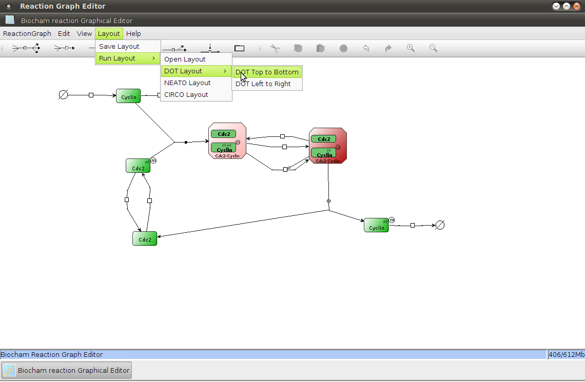
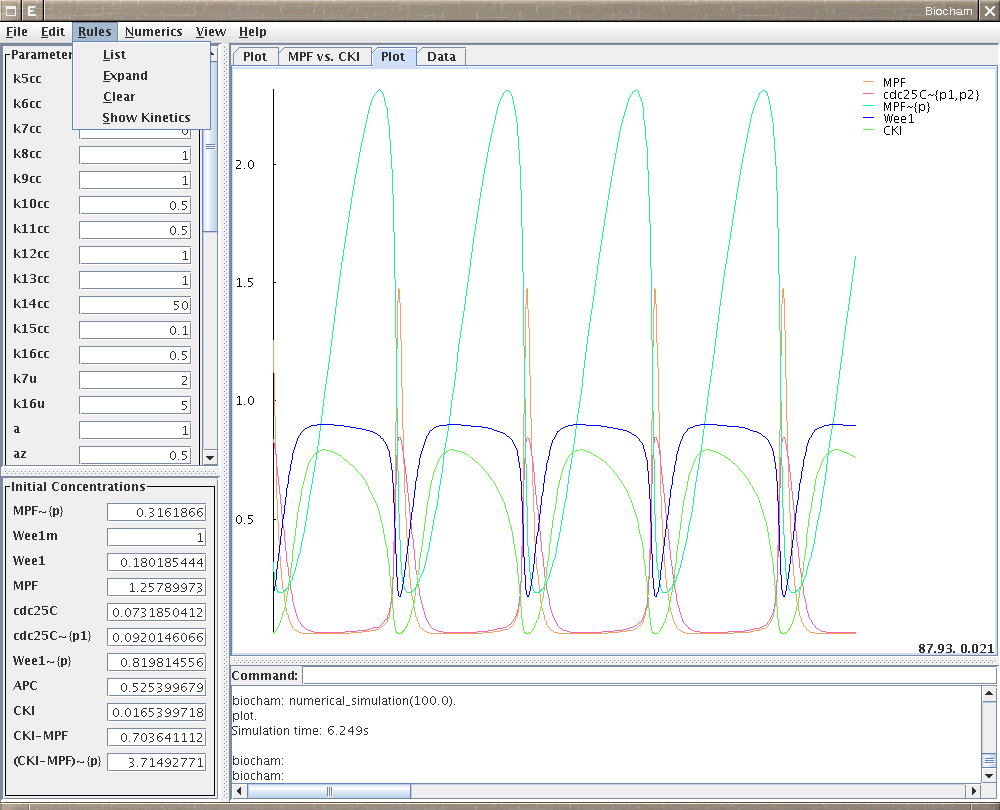
Most commands are directly accessible from the Graphical User Interface with buttons, and even the reaction rules can now be defined graphically with a graphical editor. Training in Biocham can thus be started directly with the GUI by opening the examples of Biocham models, and trying the different features provided in the menus. The structure of the menus in the GUI roughly follows the structure of chapter 4 (Biocham commands) of this reference manual.

Chapter 2
Syntax of Biocham Reaction Systems

2.1  Constituents of a Biocham Model

A Biocham model is composed of a list of plus optionnally:
The rule-based language of Biocham is compatible with the Systems Biology Markup Language SBML.

2.2  Biochemical objects

Biocham manipulates formal objects which represent chemical or biochemical compounds, ranging from small molecules to macromolecules, protein complexes and genes. Biocham objects can be used also to represent control variables and processes. The syntax of Biocham objects is defined by the grammar given in Table 2.1.
object molecule | molecule::namelocated molecule
molecule
name
| molecule-moleculemolecular complex
| molecule~{name,...,name}modified molecule
| gene
| ( molecule )
gene = #name
Table 2.1: Syntax of molecular objects.
A name is a word of alphanumerical and '_' characters beginning with a letter. name applies to:
Molecules can be located in a symbolic location using the :: operator, otherwise the molecule is supposed to be in the default location. The syntax of a molecule has four forms.
  1. The first form is the simplest and the most flexible one. It concerns the case in which a molecule is simply given a (case sensitive) name.
  2. The second form serves to denote multimolecular complexes with the linking operator This binary operator is assumed to be associative and commutative, hence the order of the elements in a complex does not matter. In the cases where one would like to distinguish between different orders of association, one should give names to the different complexes.
  3. The third form serves to write modified forms of molecules, by attaching the set of modified sites of the protein with the operator ~, like the set of phosphorylated sites for example. Several sets can be attached, the union is considered. The order of the elements is irrelevant.
    Example 1 cdk1, cdk1-cycB and cdk1~{tyr15,thr161}-cycB are valid notations for, respectively, the cyclin dependent kinase 1, the complex cdk1 cyclin B, and the phosphorylated form at phosphorylation sites tyrosine 15 and threonine 161 of cdk1 in the complex cdk1-cycB.
    (cdk1-cycB)~{tyr15,thr161} is another notation for the same phosphorylated form of the complex without specifying the constituent which is phosphorylated. Note that in this syntax, the complex (cdk1-cycB)~{tyr15,thr 161} is considered as formally different from cdk1~{tyr15,thr161 }-cycB.
  4. The fourth syntactical form is used to denote genes or gene promotor s, with a name beginning with # . These objects are assumed to be unique, which has a consequence on the way reactions involving such objects are interpreted by Biocham (see below).
Example 2 DMP1-#p19ARF can be used to denote the binding of protein DMP1 on the promotor of the gene producing protein p19ARF noted #p19ARF.

2.3  Reaction and transport rules

Biocham reaction rules are used primarily to represent biochemical reactions and transport. They can also be used to represent state transitions involving control variables, or to represent the main effects of complete subsystems such as protein synthesis by DNA transcription without necessarily introducing RNAs in the model. The syntax of Biocham rules is defined by the grammar given in Table 2.2.
reaction kinetics for basic_reaction
| basic_reaction
| name : basic_reaction
| name : kinetics for basic_reaction
basic_reaction =solution => solution.
| solution =[object]=> solution.
| solution =[solution => solution]=> solution.
| solution <=> solution.
| solution <=[object]=> solution.
solution _ | object | integer*object | solution + solution | ( solution )
kinetics simple_kinetics
| (simple_kinetics , simple_kinetics)
| if condition then simple_kinetics
| if condition then simple_kinetics else simple_kinetics
| if condition then simple_kinetics else (kinetics)
simple_kinetics =[object]
| float
| name
| simple_kinetics * simple_kinetics
| simple_kinetics / simple_kinetics
| simple_kinetics + simple_kinetics
| simple_kinetics - simple_kinetics
| simple_kinetics ^ simple_kinetics
| min( simple_kinetics , simple_kinetics)
| max( simple_kinetics , simple_kinetics)
| abs( simple_kinetics )
| log(simple_kinetics)
| exp(simple_kinetics)
| cos(simple_kinetics)
| sin(simple_kinetics)
| floor(simple_kinetics)
| frac(simple_kinetics)
| MA(simple_kinetics)
| MM(simple_kinetics, simple_kinetics)
| H(simple_kinetics, simple_kinetics, simple_kinetics)
| random
| (simple_kinetics)
condition simple_kinetics < simple_kinetics
| simple_kinetics > simple_kinetics
| simple_kinetics = simple_kinetics
| simple_kinetics =< simple_kinetics
| simple_kinetics >= simple_kinetics
| condition and condition
| true
Table 2.2: Syntax of reaction rules.
A solution is a multiset of molecular objects written as a linear expression, e.g. 2*CycA+CycB. The character _ denotes the empty solution.
In a reaction rule, a molecule appearing in both the left and right-hand sides of the rule with the same stoichiometric coefficient is called a catalyst of the reaction. As a syntactical shorthand, one catalyst molecule can be written between square brackets in the arrow.
Example 3 The rule
cdk1-cycB =[Myt1]=> cdk1~thr14-cycB.
is a phosphorylation rule with catalyst Mytosine 1. This rule is equivalent to
cdk1-cycB + Myt1 => Myt1 + cdk1~{thr14}-cycB.
Similarly a catalyst reaction can be written between square brackets in the arrow of the rule (see example 6). When a reaction rule has several catalysts
There is a warning if a reaction can proceed with a null concentration for one of its reactant. There is also a warning if a molecular species appears in the kinetic expression of a reaction without appearing as reactant. It is worth noticing that the syntax of reaction does not have a proper place for inhibitors which appear in the kinetic expression as divisors. We recommend to write the inhibitors of a reaction as catalysts the rule.
In the Boolean semantics of Biocham models where one reasons on the presence and absence of molecules over time, both the multiplicity (stoichiometry) of molecules in a solution and the reaction kinetics are ignored. In such a Boolean abstraction, a reaction transforms one solution matching the left-hand side of the rule, in another solution in which the objects of the right-hand side have been added. The molecules in the left-hand side of the rule which do not appear in the right-hand side are non-deterministically present or consumed in the resulting solution. This convention reflects the capability of Biocham to reason about all possible behaviors of the system with unknown kinetic parameters [1,2,3]. Following the uniqueness assumption, molecules marked as "genes" with the '#' notation, or any compound built on such a molecule (such as DMP1- #p19ARF for instance) are not multiplied. These objects remain unique and are deterministically consumed in the form in which they appear in the left-hand side of the rule.
In the differential semantics and respectively the stochastic semantics of Biocham, the kinetic expressions the reaction rules are used to associate to a Biocham model an ordinary differential equation (ODE), respectively a continuous-time Markov Chain (CTMC). If a rule is provided without kinetic expression, a mass action law kinetic with reaction rate 1 is assumed, i.e. MA(1).
Compound concentrations are allowed between square brackets in kinetic expressions, e.g. [cycB]. When a name is given in a kinetic expression, a corresponding parameter or macro will be looked for. A special parameter with name Time gives the current value of time during a numerical simulation. The exponential notations 1e6 or 7.2E-4 are accepted.
The abbreviations MA , MM and H represent respectively Mass Action law , Michaelis-Menten and Hill kinetics In the first case, the parameter given as argument will be multiplied by all reactants' concentrations to provide the kinetic law.
Example 4 MA(0.001) for cdk1 + cycB => cdk1-cycB. is a complexation rule with mass action law kinetics and constant rate 0.001. It is equivalent to the rule
0.001*[cdk1]*[cycB] for cdk1 + cycB => cdk1-cycB.
In the second case the two arguments represent the Vm and Km of the Michaelian kinetics; the law will have the form: Vm*[S]/(Km+[S]), where S is the single reactant (an error is raised if the reaction contains several reactants, in particular the enzyme which is supposed constant should not appear as catalyst of the reaction). The command expand_rules will show the expanded kinetics.
In the third case, H(Vm,Km,n) = Vm*[S]\^n /(Km\^n+[S]\^n), the first argument Vm represents the maximum value, Km the threshold, n the order of Hill function and [S] is the concentration of the single reactant (an error is raised if the rule contains several reactants). The order can be any real valued expression.
Pairs of kinetic rates are given for reversible reactions.
Example 5 The rule (1*[RAF]*[RAFK],0.4*[RAF-RAFK]) for RAF + RAFK <=> RAF-RAFK. is a reversible complexation rule given with a pair of kinetic rates: the product of the concentrations for the complexation, 0.4 times the complex concentration for the decomplexation, which is equivalent to the pair (MA(1), MA(0.4)).
A kinetic expression may also contain a conditional expression , where the condition is a conjunction of linear (in)equations.
Example 6 if [X] > 0.8 then k for X =[ATP => ADP]=> Y represents a reaction, only able to proceed when there is enough X and such that X is transformed into Y by consuming energy from ATP. cdk1::nucleus=>cdk1::cytoplasm is a transport rule of cdk1 from the nucleus to the cytoplasm.
In presence of conditional expression in kinetic expression, the differential semantics of a Biocham model is not an ODE but a hybrid automaton , i.e. an hybrid system with different ODE dynamics in a finite number of phases.
The random function is provided for convenience but should normally not be used. It generates uniformly distributed pseudo-random real numbers in the interval [0,1[. The random generator seed is reinitialized by the seed command.

2.4  Events

An event makes it possible to modify the values of one or several parameters once a particular condition is satisfied. Events are effective in numerical simulations only. They allow us to implement a restricted form of hybrid automata which the continuous variables are not modified by the automaton.
event = | event(condition,name,kinetics)
| event(condition,[name,...,name],[kinetics,...,kinetics])
time_event = | time_event(kinetics,condition,name,kinetics)
| time_event(kinetics,condition,[name,...,name],[kinetics,...,kinetics])
Table 2.3: Syntax of events.
A Biocham event is composed of one condition, a list of parameters and a list of values. A time event adds the condition that time be equal to some expression. The implementation of time events is more efficient but requires that the expression for time does not depend on concentrations of objects.
See Section 4.2.2 for more details.

2.5  Object and rule patterns

Patterns are used to define sets of objects or rules in a concise manner. Patterns can be used to specify the initial state, the reaction rules, or particular sets of objects, rules or temporal formulae passed as arguments in various Biocham commands. Patterns introduce the special character ? and variables noted with a name beginning with '$', to denote unspecified parts of a molecule. The parts of the molecules matched by ? or a variable can be empty.
The syntax of patterns for objects is defined in Table 2.4.
object_pattern molecule_pattern | molecule_pattern::simple_pattern
variable ? | $name
simple_pattern =name | variable
molecule_pattern =simple_pattern
| molecule_pattern-molecule_pattern
| molecule_pattern~{simple_pattern,...,simple_pattern}
| molecule_pattern~variable
| gene
| ( molecule_pattern )
Table 2.4: Syntax of patterns for objects.
Example 7 cdk1~? is a pattern representing cdk1 itself and any phosphorylated form of it. cdk1~{tyr15,?} or equivalently cdk1~{tyr15}~? represents any form of cdk1 phosphorylated on tyrosine 15 at least. cdk1-? represents cdk1 itself and any complex containing cdk1. cdk1~?-? is a pattern representing all forms of cdk1, phosphorylated and/or complexed.
When patterns are used to define the initial state or some reaction rules (e.g. with the command add_rules), the variables that appear in the pattern have to be given a range of possible values, by using the where construct. When patterns are used to match rules, like in the list_rules or delete_rules command, the where construct cannot be used. The character ? can match any solution (even empty). The syntax of patterns for rules is given in Table 2.5.
reaction_pattern kinetics_pattern for basic_reaction_pattern where constraints
| basic_reaction_pattern where constraints
| reaction_shortcut
basic_reaction_pattern =name : basic_reaction_pattern
| solution_pattern => solution_pattern.
| solution_pattern =[object_pattern]=> solution_pattern.
| solution_pattern =[solution_pattern => solution_pattern]=> solution_pattern.
| solution_pattern <=> solution_pattern.
| solution_pattern <=[object_pattern]=> solution_pattern.
solution_pattern variable | object_pattern | integer * object_pattern
| solution_pattern + solution_pattern | (solution_pattern)
constraints constraints and constraints
| variable in {object_pattern,...,object_pattern}
| variable not in {object_pattern,..., object_pattern}
| variable in all
| variable in all_simple
| variable in parts_of{ name, name,... }
| name not in variable
| variable diff object_pattern
| variable phos_form object_pattern
| variable not phos_form object_pattern
| variable more_phos_than object_pattern
| variable not more_phos_than object_pattern
| variable submol object_pattern
| variable not submol object_pattern
| variable has_simple_mol_in_common object_pattern
| variable has_no_simple_mol_in_common object_pattern
kinetics_pattern =same as 'kinetics' but with 'molecule_pattern' instead of 'molecule'
reaction_shortcut =complexation
| decomplexation
| re_complexation
| phosphorylation
| dephosphorylation
| re_phosphorylation
| synthesis
| degradation
| elementary_interaction_rules
| more_elementary_interaction_rules
| more_elementary_interaction_rules(object)
Table 2.5: Syntax of patterns for rules.
The in constraint is set membership. The set all (resp. all_simple ) refers to all the molecules already known by the system, i.e. (resp. limited to non-localized, non-complexed and non-phosphorylated forms). This means that using these constructs makes the semantics of the rule dependent on the context (order of rules, model parts loaded before, etc.), and is thus recommended only to advanced users.
The diff and not in have the opposite meaning (the variable cannot take the given value(s)). For instance $A not in {$B,per} means that $A represents a molecule which cannot be per, not have the same value as $B. The second case of not in corresponds to the absence of some phosphorylation site (the name) in a set of phosphorylated sites (the variable). See the example below.
The phos_form constraint, forces the variable and the object_pattern to differ only by some phosphorylations. more_phos_than forces the variable to be more phosphorylated than the object_pattern.
The submol constraint forces the variable to be a sub-molecule of the pattern, the has_simple_mol_in_common constraint imposing a common sub-molecule.
When using constraints relating a variable to an object_pattern, variables appearing in that object_pattern have to be constrained beforehand. Moreover, to define a variable range (for instance to add a rule), one has to use for each variable at least one positive constraint: in or sub_mol, and if the adequate declaration exists, phos_form or more_phos_than.
Example 8 The reaction pattern (cdk1~?-? + ? => ?) will match all rules reacting with any form (phosphorylated or complexed) of cdk1. The pattern (? =[Myt1]=> ?) matches all rules involving the catalyst Myt1. This pattern will match all the rules having Myt1 in their left and right-hand sides, even if they were not written with the catalyst notation. This pattern cannot be used to define reaction rules since it can match unconstrained molecules.
Example 9 The reaction pattern cdk46~$P + $cycD => cdk46~$P-$cycD
 where $cycD in {DMP1~?-cycD~?, cycD~?}. will match all complexation rules of all phosphorylated forms of cdk46 with all phosphorylated forms of cycD or DMP1-cycD. This pattern can be used to define reaction rules. All possible phosphorylated forms of molecules cdk46, DMP1 and cycD have to be declared however (see section below) in order to constrain the variable $P and the different occurrences of ?. Note that if the three molecules in this pattern had three phosphorylation sites each, they would have 23=8 forms each, thus the pattern would specify 8×(8×8+8)=576 reaction rules! Reaction patterns must thus be used with care for specifying reaction rules and only the relevant phosphorylation sites should be declared for a molecule.
Example 10 The reaction pattern cdk1~$P-$cyc =[Wee1]=> cdk1~$P~p2-$cyc
 where p2 not in $P and $cycA in {cycA, cks1-cycA}
 and $cyc in { $cycA, cycB, cycB-cks1}. specifies the phosphorylation on site p2 of several cdk1 complexes not already phosphorylated on p2. This pattern can be used to define reaction rules. If cdk1 is declared with 3 phosphorylation sites {p1,p2,p3}, there are 4 forms not containing p2 to combine with the 4 possibilities for the variable $cyc. This reaction pattern thus expands into 16 reaction rules.
The reaction short-cuts stand for the following reaction patterns:
complexation :
$A + $B => $A-$B where $A in all and $B in all and $A diff $B
decomplexation :
$A-$B => $A+$B where $A in all and $B in all and $A diff $B
re_complexation :
$A + $B <=> $A-$B where $A in all and $B in all and $A diff $B
phosphorylation :
$A =[$C]=> $B where $A in all and $B in all and $C in all
 and $B more_phos_than $A and $A diff $B
dephosphorylation:
$A =[$C]=> $B where $A in all and $B in all and $C in all
 and $A more_phos_than $B and $B diff $A
re_phosphorylation :
$A <=[$C]=> $B where $A in all and $B in all and $C in all
 and $B more_phos_than $A and $A diff $B
synthesis :
_=[$G]=>$A where $A in all_simple and $G in all and $A diff $G
degradation :
$A =[$D]=>_ where $A in all and $D in all and $A diff $D
elementary_interaction_rules : either complexation, decomplexation,
or phosphorylation, dephosphorylation, synthesis, degradation
more_elementary_interaction_rules : same as above plus combinations
more_elementary_interaction_rules(object) : forces the use of the given object in the rules.
Finally, the set of all possible modified forms of a given molecule can be declared by associating to the molecule the set of sets of sites which can be modified (e.g. phosphorylated). In these declarations, the function parts_of can be used to denote all subsets of a set. These declarations are not mandatory, except for defining rules with patterns containing phosphorylation variables.
Example 11 the declaration add_declaration(cdk2~{{},{p1},{p2},{p1,p2}}). specifies that cdk2 has two phosphorylation sites p1, p2 and that all combinations are possible. This declaration is equivalent to add_declaration(cdk2~parts_of({p1,p2})).
The purpose of declarations is to constrain implicitly the domain of modification variables which appear in molecule patterns. Only modification sites can be declared. In a reaction pattern used for defining reaction rules, the other variables, such as complexation variables, must thus be explicitly constrained in the where part of the pattern.
Declarations can be entered also at top-level with the command declare, can be listed with the command list_declarations and can be cleared with the command clear_rules. Since the aim of declarations is to define the possible modification sites, any rule where a molecule appears in a form in contradiction with its declaration is ignored (with an error message). Since most molecules appear also in non-phosphorylated form, a warning is given when a declaration excludes the empty set.

Chapter 3
Syntax of Biocham Temporal Specifications

Biocham uses a second language for specifying temporal behaviors of a system. This original feature of Biocham which can be used
The temporal specification language is based on temporal logic and comes with two versions: a Boolean version and a numerical version.

3.1  Boolean temporal properties

In Biocham, temporal Boolean properties of a system can be formalized at a very high level of abstraction in propositional Computation Tree Logic (CTL). These temporal formulae can be used to query reachability properties in the model independently of the kinetics, in particular when the kinetics are not known or for querying possibly rare stochastic behaviors. They can also be used as constraints to revise the model.
In CTL, Boolean propositions are used to describe states of the system, with respect to the absence or presence of molecular compounds.
Example 12 For instance, the formula cdk1 & MPF & !(cdk7-cycH) represent the states of the system where cdk1 and MPF are present and cdk7-cycH is absent, the rest being undetermined.
CTL is an extension of propositional logic to express formulae on the evolution of states over time. CTL introduces two path quantifiers for non-determinism: E, A, and several operators for time: F, G, X, U. The path quantifier E presses the existence of a path, A means for all paths, F means at some time point (on the path), G means at all time points, X means at the next time point, U is a binary operator meaning that a formula is true until a second formula becomes true.
Furthermore, since it is possible to have an initial state only partially defined (the molecules may be present, absent, or their presence is unspecified), a Biocham temporal Boolean formula is prefixed with an initial state quantifier. There are two such quantifiers: Ei and Ai , meaning respectively, "there exists an initial state" and "for all initial states". The syntax of CTL with initial state quantifiers is defined by the grammar ictl given in Table 3.1.
ictl =Ei(ctl) | Ai(ctl)
ctl=object
| (ctl)
| EF(ctl)
| AF(ctl)
| EG(ctl)
| AG(ctl)
| E(ctl U ctl)
| A(ctl U ctl)
| E(ctl W ctl)
| A(ctl W ctl)
| EX(ctl)
| AX(ctl)
| !(ctl) negation
| ctl & ctl conjunction
| ctl | ctl disjunction
| ctl xor ctl exclusive or
| ctl -> ctl implication
| ctl <-> ctl equivalence
| reachable(ctl) same as EF(ctl), i.e. on some path the formula can become true
| stable(ctl) same as AG(ctl), i.e. on all paths the formula remains always true
| steady(ctl) same as EG(ctl), i.e. on some path the formula is always true
| checkpoint(ctl,ctl) same as !(E(!(ctl1) U ctl2))) i.e. there is no path where
the first formula is false until the second is true
| loop(ctl,ctl) same as AG((ctl1->EF(ctl2))\&(ctl2->EF(ctl1))) approximates
the oscillation property where two formulae are alternatively true.
| oscil(ctl) same as loop(ctl,!(ctl)) approximates the oscillation property
where a formula is alternatively true and false
Table 3.1: Syntax of propositional CTL properties.
Example 13 Ei(EF(cycB)) expresses the existence of an initial state such that there exists a path on which at some time point cycB is present. Ai(AF(cycB)) expresses that for all initial states and on all paths, cycB is finally present at some time point.
Ai(!(E(!(cdc25) U cdk1-cycB))) checks that cdc25 is a checkpoint for the activation of MPF (the unphosphorylated form of the cdk1 cycB complex) for all initial states, that is there does not exist a path on which cdc25 is always absent until the complex cdk1-cycB is present.

3.2  Numerical temporal properties

In Biocham, temporal quantitative properties about concentrations and their derivatives can be formalized as well in Linear Time Logic with numerical constraints over the reals, noted LTL(R) The syntax of LTL(R) formulae is defined by the grammar in Table 3.2.
ltl = condition (*)
| (ltl)
| F(query) finally
| G(query) globally
| X(query) next
| ltlUltl until
| !(ltl) negation
| ltl & ltl conjunction
| ltl | ltl disjunction
| ltl xor ltl exclusive or
| ltl -> ltl implication
| ltl <-> ltl equivalence
| oscil(molecule, int) oscillations
| oscil(molecule, int, float)
| period(molecule, float) periodic oscillations
| phase_shift(molecule, molecule, float) phase delay
| cross(molecule, molecule, int) repetitive crossing
| curve_fit(list_of_molecules,list_of_floats,list_of_names) curve fitting
| formulae with dedicated solver (**)
(*): In the conditions here, the derivatives of the concentrations can also appear with the syntax: d([Molecule])/dt.
(**): The formulae with dedicated solvers are listed in Tables 3.3 and 3.4.
Table 3.2: Syntax of first-order LTL(R) properties.
First-order LTL(R) formulae (FOLTL(R) ) may contain free variables in the conditions which, in this case, are restricted to be linear inequalities (otherwise they may contain any mathematical expression). Those variables are real-valued. They are written with a word of alphanumerical characters beginning with a lowercase letter. Their names must differ from kinetic parameters and macros.
Example 14 G(([RAF-RAFK] >= [RAF~{p1}]) U (d([RAF])/dt < 0.3)) expresses that all along the simulation trace, the concentration of the RAF-RAFK complex is greater than that of phosphorylated RAF, until the derivative of the concentration of RAF becomes lower than 0.3.
The formula oscil (M,n) is an abbreviation for n successive alternations of the sign of d([X])/dt.
oscil(M,n,V) states that M oscillates, with a maximum value greater than V, at least n times.
Example 15 oscil(cycB,3) expresses the fact that, along the trace, the concentration of cycB goes up and down twice.
period (M,p) states that molecule M oscillates at least 3 times (with the above meaning) and has period p (with 4% error) for the last three oscillations. phase_shift (M,N,s) states that there is delay of s between the (last three) peaks of M and those of N.
cross (M1,M2,n) is an abbreviation for n successive repetitions of crossings between the concentration values of [M1] and [M2].
curve_fit (list_of_molecules,list_of_floats,list_of_names) is an abbreviation for a curve fitting FOLTL(R) formula, stating that each molecule, at a given time, is equal to a particular value or variable. The three lists must be of the same length,
Example 16 curve_fit([A,A],[10,50],[v1,v2]).
stands for the FOLTL(R) formula G((Time=10 -> [A]=v1) & (Time=50 -> [A]=v2)) giving the values of A at time 10 and 50 in free variables v1 and v2.
A list of particular specifications of the form specification(list_of_molecules, list_of_variables) that represent useful FOLTL(R) formulae is defined, with dedicated solvers for efficient computation of the corresponding validity domains and their combination with other temporal logic constraints.
Example 17 distanceSuccPeaks([A],[d]) constrains variable d to be the value of one time distance between two successive peaks of A (i.e. d is a period value).
Name and description Equivalent formula Validity domain D computed by the specific solver
Table 3.3: List of LTL(R) formulae with dedicated solvers (1/2)
Name and description Equivalent LTL(Rlin) formula Validity domain D computed by the specific solver
Table 3.4: List of LTL(R) formulae with dedicated solvers (2/2)

Chapter 4
Commands at Top-level

The command biocham starts the Biocham interpreter. Some Biocham files can be passed as arguments to the command to be loaded immediately. Under the Biocham prompt, the following commands are available, they must be terminated by a dot. The previous typed commands can be retrieved by pressing ctrl-p or up-arrow. The commands can be automatically completed by pressing on the tabulation key. A command can be interrupted by ctrl-c and a (abort).
Some commands take a list as argument. Lists are noted between square brackets, e.g. [a,b,c]. Sets are noted between braces, e.g. {a,b,c}. To quit the interpreter type quit.
quit .
quits the interpreter.
prolog('goal') .
this extra command executes a Prolog (the programming language in which Biocham is implemented) goal passed as a string in the argument. This command is documented for the sake of completeness but should not be useful. It is disabled in Biocham-web.
seed(int) .
initializes the random number generator seed.

4.1  Loading, listing and exporting models

Biocham files are written in a file suffixed by '.bc'. Biocham files may contain:
A parametric Biocham model may be defined in a file containing only reaction rules. Then different models may be derived from the parametric model by adding commands for defining different parameter values or different initial states.
Biocham models can also be imported from (or exported to) files in different formats including SBML, xppaut ODE and graphical notations.
Files and directories can be designated with absolute or relative path names with respect to the current directory which may be changed with the following commands:
current_directory .
displays the current directory.
change_directory(input_file) .
changes the current directory.

4.1.1  Biocham files

load(input_file) .
acts as the corresponding load_biocham / load_sbml / load_ode / load_trace, depending on the file extension (respectively .bc, .xml, .ode, .csv - assuming no extension is .bc)
add(input_file) .
acts as the corresponding add_biocham / add_sbml / add_ode, depending on the file extension (respectively .bc, .xml, .ode - assuming no extension is .bc)
clear_biocham .
clears the current model.
load_biocham(input_file) .
clears the current model, loads the reaction rules and executes the commands (with the file directory as current directory) contained in the given Biocham .bc file.
Example 18 load_biocham('cell_cycle.bc') or load_biocham(cell_cycle). Note that in the latter form, the quotes are not necessary and the suffix is automatically added to the name.
add_biocham(input_file) .
the rules of the given .bc file are loaded and added to the current set of rules. The commands contained in the file are executed (with the file directory as current directory).
list_model .
lists the current Biocham model.
export_biocham(output_file) .
saves the current Biocham set of rules, macros, parameters and initial state in a .bc file.
expand_biocham(input_file) .
saves the current Biocham set of rule instances, macros, parameters and initial state in a .bc file where all reaction rule patterns are expanded.
export_init(output_file) .
saves the current initial state, macros and the value of parameters in a .bc file.
export_param(output_file) .
saves the current values of parameters (only) in a .bc file. This command might be useful when several parameter sets are associated to the same set of rules.

4.1.2  SBML files

export_sbml(output_file) .
exports the current Biocham set of rules (including kinetic laws) and initial state to an SBML .xml file. Molecules are translated by removing all '-' and '~{','}'.
export_sbml3(output_file) .
exports the current Biocham set of rules (including kinetic laws) and initial state to an SBML Level 3 version 1 core .xml file. Molecules are translated as above.
load_sbml(input_file) .
add_sbml(input_file) .
act as the corresponding load_biocham/add_biocham commands but importing reactions, parameters and initial state (and only that!) from an SBML .xml file.
curate_sbml(input_file) .
curate automatically the writing of the ODE model from an SBML .xml file, replacing existing file (see curate_model).
curate_sbml(input_file, output_file) .
curate automatically the writing of the ODE model from an SBML .xml file (file1), outputing to file2 (see curate_model).

4.1.3  ODE files

export_ode(output_file) .
exports the ODE associated to the current Biocham model, with parameters, macros and initial state, to an ASCII xppaut .ode file. Molecules are translated by removing all - and ~{,} and if necessary shortening the resulting name.
export_ode_latex(output_file) .
exports the ODE as above to an ASCII .tex file in LaTeX format (suitable for inclusion with the LaTeX command \include{file}). Molecules are translated by removing all - and ~{,} characters.
load_ode(input_file) .
clears the current model and creates a new Biocham model (reaction rules, initial state, parameters and macros) inferred from an xppaut .ode file (preferably written with parameters). As any ODE may not correspond to a well-formed reaction rule model, the reaction rules inferred from the ODE may raise warnings (e.g. about an inhibitor appearing in the kinetic expression of a reaction but not appearing as a reactant of the reaction).
add_ode(input_file) .
adds the Biocham rules (plus initial state, parameters and macros) inferred from an xppaut .ode file.
curate_model .
use the system of ODE from the current model as input to compute a system of reactions with the same ODE semantics, by inferring well-formed reactions whenever possible. []

4.1.4  Graphics files

export_dimacs(output_file) .
exports the current Biocham set of reactions as a regular graph in the dimacs standard format for graphs (.col file).
export_dot(output_file) .
exports the current Biocham set of rules and initial state into a .dot file. That file can then be used to generate pictures of the reaction graph, with for instance tools of the Graphviz suite.
if you simply want to visualize the output and have both Graphviz and gv installed, see the dot command below.
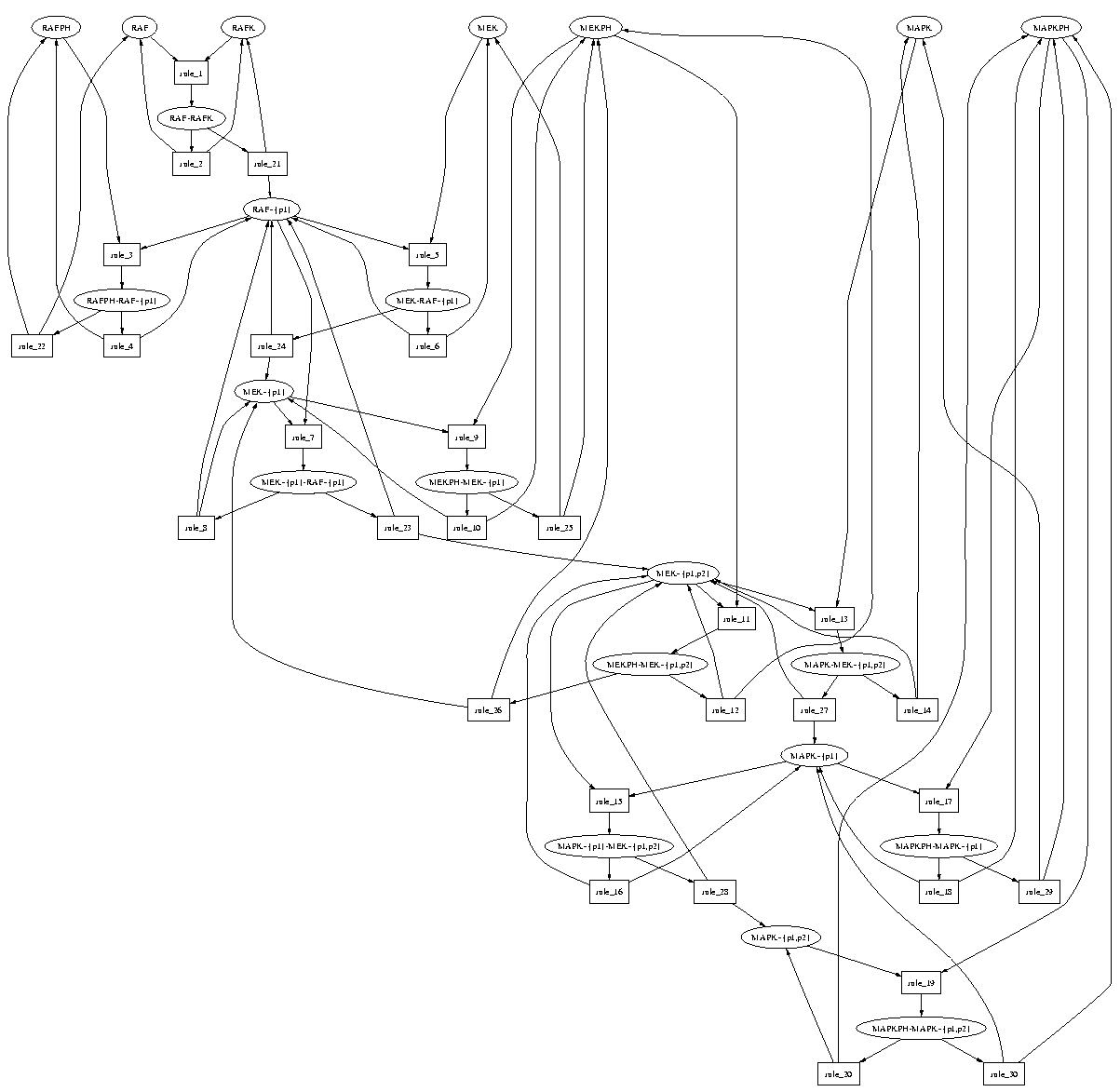
Example 19 The Unix command dot -Tpng file.dot > file.png will generate a PNG image of the map. For instance, the reaction graph of EXAMPLES/MAPK/mapk.bc will be depicted as follows
mapk_dot.png
export_dot(output_file, utypelist_of_options) .
exports the current Biocham set of rules and initial state into a .dot file (see above). The list of options can contain: init_up, to force the molecules present in the initial state to be shown on the top of the image (see example above); mod\_double, to show enzymes catalyzing a reaction or modifiers of some kind (i.e. both input and output) with a double arrow (input/output) instead of a simple dashed arrow; col_path, to color in red the latest pathway returned by a CTL query; double\_size, to produce A3 sized graphs instead of the default A4; state to produce the state graph instead of the reaction graph (be careful, it can be huge!).
Example 20 export_dot(test,[init_up,mod_double,col_path]). to use all of the options, and save the result in the file test.dot;
export_dot(test,[init_up]) .
to obtain an image like that of the above example (after using dot).
dot .
draw_reactions .
visualize the graph resulting from an export_dot with no options, using both Graphviz and gv that have to be installed and in your PATH.
json_reactions .
displays the current Biocham set of reactions as a JSON object.

4.1.5  Other files

export_nusmv(output_file) .
exports the current Biocham set of rules and initial state in an SMV .smv file. Notations for molecules are translated by replacing the characters _, (, ), }, , and ~{ respectively by __, _L, _R, _r, _c and _l. Furthermore the names A, AF, AG, AX, B, E, EF, EG, EX, F, G, H, O, S, U, T, V, W, X, Y, Z and xor are prefixed by _.
export_lotos(output_file) .
exports the current Biocham set of rules and initial state in a LOTOS .lot file. Molecules are translated with the same convention as for SMV.
export_prolog(output_file) .
exports the current Biocham set of rules, initial state and temporal specification in a Prolog .pl file, where reactions are represented by a transition system between Boolean states, and where CTL properties can be evaluated with a model checker implemented in Prolog (file ctl.pl).
export_biopepa(output_file) .
exports the structure (stoichiometry matrix) of the Biocham model, i.e., the effect of each reaction on each species, as a BioPEPA model.

4.2  Listing and editing rules and events

4.2.1  Rules

list_rules .
lists the current set of rules.
list_rules(reaction_pattern) .
lists the current set of rules matching the given pattern.
Example 21 list_rules(? => cycA~?-? + ?) will list all the rules containing any form of cycA in the right hand side.
expand_rules.
lists all the instances of the current set of rules, with the associated rule number.
expand_rules(reaction_pattern) .
lists all the instances of the current set of rules matching the given pattern.
add_rules(reaction_pattern) .
add_rule(reaction_pattern) .
add_rules(set_of_reaction_patterns) .
add_rule(set_of_reaction_patterns) .
adds reaction rules to the current set of rules.
delete_rules(reaction_pattern) .
delete_rules(set_of_reaction_patterns) .
deletes all reaction rules matching one pattern from the current set of rules. Warning: currently, if a kinetics pattern is provided, it will be ignored.
clear_rules .
clears the current set of rules and all molecule declarations.
rule(integer) .
rule(reaction_name) .
shows the n-th rule (after expansion), or the rule(s) with the corresponding name (i.e. of the form reaction_name : A => B).
pathway(list_of_integers) .
pathway .
show the rules of corresponding numbers (after expansion). If no list is given and the trace corresponding to a query has been generated, then use the list given by that trace as argument.
list_ODE .
returns the set of ordinary differential equations and initial concentrations (one line per molecule).
list_ODE(molecule) .
Same as above but only for the given molecule.

4.2.2  Events

add_event(condition,parameter,kinetics) .
add_event(condition,list_of_parameters,list_of_kinetics) .
sets up an event that will be fired each time the condition given as first argument goes from false to true. This command is effective in numerical simulations only. Upon firing, the parameter(s) given as second argument receives a new value computed from the third argument. The initial values of the parameters are restored after the simulation.
Example 22 parameter(N,1). add_event([X]>=2.0,N,1-N). Each time [X] goes above the threshold value 2.0, N will become 1-N. At the end of the simulation, N is reset to 1.
add_time_event(kinetics,condition,parameter,kinetics) .
add_time_event(kinetics,condition,list_of_parameters,list_of_kinetics) .
sets up an event at a fixed time given by the first argument. It will be fired if the condition given as second argument is true.
Example 23 add_time_event(2.0,true,N,1-N).
is logically equivalent to, but more efficient than,
add_event(Time>=2.0,N,1-N).
delete_event(condition,parameter,kinetics) .
delete_event(condition,list_of_parameters,list_of_kinetics) .
delete_time_event(kinetics,condition,parameter,kinetics) .
delete_time_event(kinetics,condition,list_of_parameters,list_of_kinetics) .
removes an existing event.
delete_events .
deletes all the declared events.
list_events .
lists all the declared events.

4.2.3  Hybrid boolean-differential models

As described in ??? it is possible to automatically add the events describing the hybrid automaton obtained from the composition of a boolean and a differential model. The differential model is entered as usual (see Section 4.2.1). The boolean states and transitions are defined as follows:
add_boolean_state(int, list_of_boolean_variables) .
The list of boolean variable names describes the boolean variables that should be set to true in the state numbered by the int.
set_initial_boolean_state(int) .
Sets the initial state to the state numbered by the given int.
add_boolean_transition(transition, int, int) .
Defines a transition with given name, from the state corresponding to the second argument to the state corresponding to the third.
An interface allows to put conditions on the variables of the differential model for the boolean transitions. These are compulsory in order to relate logical time and continuous time.
add_interface(transition, condition, list_of_parameters, list_of_kinetics) .
Adds condition given as second argument to the boolean transition with name equal to the first argument, actions (assignments) similar to those of events can also be provided (see 4.2.2).

4.2.4  Hybrid stochastic-differential models

Similarly, it is possible to compose a stochastic model, with SSA implemented as events and a continuous model through the following commands:
compose_ode_stochastic(ODE file, SSA file, Output file, volume, time) .
Composes in the Output file a biocham model combining the two input files. The fourth argument represents the volume used for the conversion and the last one the duration of an initial simulation.
compose_ode_stochastic(ODE file, SSA file) .
Same as above but with default values of 'out.bc', 1 and 200.

4.3  Listing and defining initial states, molecules and locations

4.3.1  Initial state

The initial state can be partially defined by giving the list of objects which are present in the initial state and the list of objects which are absent from the initial state. The other objects can be present or absent. When no precision is given, present objects are given a default concentration of 1.
list_initial_state .
lists the objects which are present (including their initial concentration) and absent from the initial state.
list_all_initial_states .
same as above but lists undefined objects as well.
clear_initial_state .
makes undefined all objects possibly present or absent in the initial state. Also deletes all parameters and macros.
present(object_pattern) .
present(set_of_object_patterns) .
all objects (appearing in the instances of the current set of rules) and matching one of the given object patterns are made present in the initial state.
Example 24 present({cycA, cdk1, cycE~?}). makes cycA, cdk1 and all modified forms of cycE present in the initial state.
present(object_pattern,concentration) .
present(object_pattern,parameter) .
initializes the given objects with the given initial concentration, or sets it to be equal to the value of the given parameter. An initial value equal to 0 means absent.
Example 25
present(MAPK,0.3). present(CycE, k).

makes present two molecules with concentration, respectively 0.3 and the value of parameter k.
absent(object_pattern) . • absent(set_of_object_patterns) .
makes all objects (appearing in the instances of the current set of rules) and matching one of the given object patterns, absent from the initial state. Same as present with initial concentration equal to 0.
undefined(object_pattern) . • undefined(set_of_object_patterns) .
makes all objects (appearing in the instances of the current set of rules) and matching one of the given object patterns, possibly present or absent in the initial state.
make_present_not_absent .
makes all objects (appearing in the instances of the current set of rules) which are not declared absent, present in the initial state.
make_absent_not_present .
makes all objects (appearing in the instances of the current set of rules) which are not declared present, absent in the initial state.
set_initial_state(state) .
set_initial_state(set_of_states) .
applies the given states.
Example 26
set_initial_state({present(MAPK,0.3),absent(CycE)}).

makes MAPK present in the initial state with concentration 0.3, and CycE absent.

4.3.2  Molecules

add_declaration(molecule_declaration) .
declares the set of all modified forms of a molecule. This is useful only for defining sets of reaction rules with rule patterns.
list_declarations .
lists all the declared modified forms of molecules.
delete_declaration(molecule_name) .
deletes a molecule declaration.
list_molecules .
lists the molecules contained in all instances of the current set of rules.
list_molecules(object_pattern) .
list_molecules(set_of_object_patterns) .
lists the objects (appearing in the instances of the current set of rules) and matching one of the given object patterns.
Example 27
list_molecules(cycE-?).
cycE
cycE-cdk2

list_all_molecules .
list_all_molecules(object_pattern) .
list_all_molecules(set_of_object_patterns) .
same as above but also including modification sites declarations and initial state.
check_molecules .
checks lower/upper case errors in molecule names. Then, tries to find production and degradation rules for all known molecules. For each potential problem, displays a warning.

4.3.3  Locations

Different locations for molecular compounds can be defined by giving them a name. These symbolic locations may represent cell compartments (e.g. nucleus, cytoplasm, etc.) or different cells (e.g. c11, c12, c21, c22). All molecules are localized, either explicitly with the :: operator, or implicitly in the default location.
The volumes of locations are not static and may vary over time. Transport rules which may contain molecules in different locations have their kinetics automatically normalized according to the volume of the location of each reactant.
volume(location,simple_kinetics) .
defines the volume of the location location by a numerical expression which may depend on parameters or concentrations of compounds. If no volume is provided for a location, it will be equal to 1, the volume of the default location.
volume(location) .
displays the volume (formula) of a given location.
list_volumes .
lists all the volumes of the different locations.

4.4  Listing and declaring parameters, macros and invariants

4.4.1  Parameters

Numerical parameters can be defined and used in a number of places, including kinetic expressions, initial concentrations, macros and events.
parameter(parameter,float) .
sets the value of a given parameter to the corresponding value.
parameter(parameter) .
shows the value of the given parameter.
parameter_list(list_of_parameter_declarations) .
sets the value of the given parameters to their corresponding value.
Example 28 parameter_list([(k1, 1), (k2, 10)]).
list_parameters .
shows the values of all known parameters.
delete_parameter(parameter) .
deletes a parameter.

4.4.2  Macros

A macro gives a name to an expression and can be used in any place where the expression could be used.
macro(macro,kinetics) .
macro(macro,sq_wave(name,float,name,float)) .
macro(macro,sq_wave(name,float,name,float,name,float)) .
sets the value of a given macro to the corresponding value, which will be re-evaluated each time a kinetic law is to be computed.
The special value sq_wave generates a square wave signal between the values of two parameters (given by the two names) with their respective duration (given by the two floats). When three names and durations are given, an initial stage of the first duration with the first value is executed before alternating between the next values/durations. Please note that some adaptive step integration methods will give a quite poor result when using square waves.
macro(macro) .
shows the expression associated to the given macro.
list_macros .
lists all known macros.
delete_macro(macro) .
deletes a macro.

4.4.3  Algebraic invariants, conservation laws and P-invariants

It is possible to impose some algebraic invariants , such as a mass conservation law , to the system in order to reduce the dimension of the ODE system. Such invariants can be checked from the rules (i.e. no reaction can make it false), from the kinetics (i.e. the derivative is formally proven equal to zero), or trusted from the user.
Some conservation laws , called P-invariants , can be automatically computed from the underlying Petri-net representation of Biocham reaction rules. These invariants are independent of the kinetics and only depend on the stoichiometry of the reactions. They correspond to modules of molecular compounds having the same life cycle.
conservation(set_of_object_patterns) .
conservation(list_of_molecules_with_stoichiometry) .
declares a new mass conservation law for all the molecules matched by the argument if it is a set, or for all molecules given with the corresponding weight. During a numerical simulation, one of those variables will be eliminated thanks to this conservation law. Be careful if you declare conservation laws and then plot the result of a previous simulation, the caption might not be correct. When added, the conservation law will be checked against the rules (i.e. purely from stoichiometry), if that fails against the kinetics. Since these checks are not complete, even a failure will be accepted with a warning.
Example 29 conservation({cycE-?}).
keeps the sum of the numbers of molecules of all complexed forms of cycE constant.
Example 30 conservation([A-A, 2*A]).
keeps the sum of the numbers of molecules of the dimer plus twice that of the monomer constant.
check_conservations .
checks all conservation laws against rules, and if necessary kinetics (see above).
delete_conservation(set_of_object_patterns) .
delete_conservation(list_of_molecules_with_stoichiometry) .
delete_conservations .
removes the given mass conservation law, or respectively all of them.
list_conservations .
prints out all the mass conservation laws.
search_conservations .
search_conservations(integer) .
computes and displays the P-invariants of the system up to a given size (default is 4). Such P-invariants are particular mass conservation laws that are independent from the kinetics.

4.5  Simulations

A Biocham model can be interpreted at three levels of abstraction either as: The latter interpretation is deterministic and produces a unique simulation trace, while the other two interpretations produce non-deterministic simulation traces.

4.5.1  Boolean simulator

For the Boolean simulator, all the objects with an undefined initial state are considered as absent in the initial state. The simulator prints the objects present in the successive states of the simulation. The set of objects which are printed can be specified with patterns. By default all objects are printed.
boolean_simulation .
boolean_simulation(count) .
performs a random simulation up to a given number of transitions (default is 30).
Note that because Biocham boolean models are highly non-deterministic, random boolean simulations are hardly representative of all possible behaviors. The temporal properties of Biocham models w.r.t. all possible behaviors can however be queried in Biocham in Computation Tree Logic CTL.
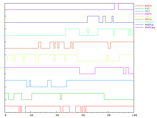
Example 31 Boolean simulation of the MAPK signaling cascade visualized with the plot command (see model EXAMPLES/MAPK/mapk.bc):
mapk.png
boolean_enumeration .
performs a step by step simulation by enumerating all possible behaviors of the system from the initial state. At each step you can either continue the simulation by typing return, backtrack to another transition by typing < , or stop the simulation by typing 'q'. The depth of the current derivation is printed.

4.5.2  ODE and stochastic simulations

The numerical simulations of Biocham models are based on the interpretation of the reaction kinetics by either ordinary differential equations or continuous-time Markov chains.
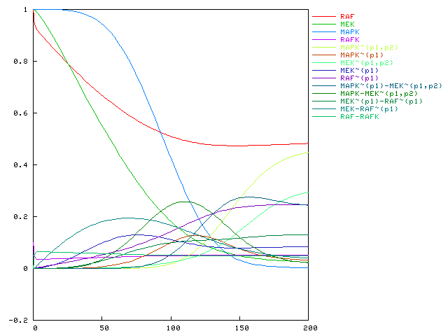
Example 32 MAPK cascade numerical simulation visualized with the plot command:
mapk_sim.png
numerical_method . shows the current numerical simulation method and its parameters (error, step_size, etc.).
numerical_method(simulation_method) .
sets the simulation method among: rk (Runge-Kutta method ), stiff (Rosenbrock's method ), ssa (Gillespie's method ) and tl (tau-leaping method ). The two first methods are for the ODE interpretation of Biocham models. The first one is a fourth-order Runge-Kutta method, with or without step-doubling (see parameters below). The second one is Rosenbrock's implicit method, with variable step-size (this is the method used by default). The latter two methods are for stochastic simulations The third one is an implementation of Gillespie's algorithm and the last one of the tau-leaping method. These methods rely on a conversion factor and a critical reaction threshold, see parameters below.
numerical_simulation .
numerical_simulation(time) .
performs a numerical simulation up to a given number of time units (default is 20).
continue(time) .
performs a numerical simulation (using one of the methods detailed below) starting from the last point of the current simulation, up to a given number of time units.

Parameters of ODE simulations:

step_size .
resets the initial step size for the Runge-Kutta method to its default value 0.01.
step_size(step) .
sets the initial step-size for the Runge-Kutta method.
step_doubling .
step_doubling(float) .
uses step-doubling method (default) to adapt the step-size to a specified maximum error (default is 0.0001).
no_step_doubling .
turns off step adaptation in Runge Kutta method (cannot be turned off for Rosenbrock method).

Parameters of stochastic simulations:

conversion_factor .
conversion_factor(integer) .
The conversion from a concentration to a number of molecules for stochastic simulations is obtained by multiplying concentration values by this conversion factor. The default value is 100 (instead of Avogadero's number). Lower conversion factors greatly speed up stochastic simulation.
critical_reaction_threshold .
prints the reaction threshold integer used in the tau-leaping method for stochastic simulations.
critical_reaction_threshold(integer) .
defines the reaction threshold integer used in the tau-leaping algorithm to determine for which reactions a tau leap is possible (default is 20).

4.5.3  Plotting the result of simulations

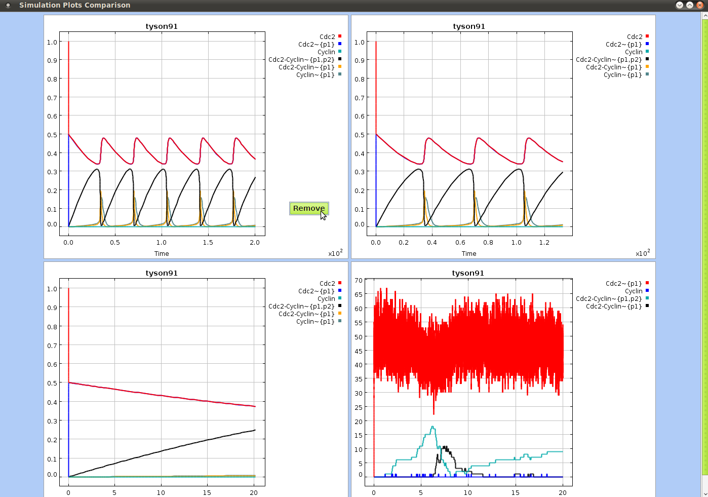
keep_plot .
keeps the current plot window open and asks future plots to use another window (for comparison).
plot .
plots the result of the last simulation, either boolean or numerical.
plot(object, object) .
plots the result of the last numerical simulation, as a trajectory in the phase space of the two given objects. The first object will be plotted on the x-axis, the second on the y-axis.
plot(object, object, object) .
plots the result of the last numerical simulation, as a trajectory in the phase space of the three given objects. The first object will be plotted on the x-axis, the second on the y-axis and the third on the z-axis.
export_plot(file_template) .
saves the numerical trace of the last simulation into two files: file_template.csv and .plot.
The .plot file may be given to GNUplot with the command load file_template.plot. The .plot file may be used to get an image by adding the commands set term png and set output "file.png" at the beginning of the .plot file.
show_molecules(object_pattern) .
show_molecules(set_of_object_patterns) .
adds the molecules matched by the pattern to the molecules printed by the simulator. Initially all molecules are shown.
hide_molecules(object_pattern) .
hide_molecules(set_of_object_patterns) .
removes the molecules matched by the pattern from the molecules printed by the simulator.
show_macros .
will plot all macros for the numerical simulator.
show_macros(set_of_macros) .
will plot at least the given macros for the numerical simulator.
hide_macros .
will hide macros for the numerical simulator.
show_parameters .
will plot all parameters for the numerical simulator and events.
show_parameters(set_of_parameters) .
will plot at least the given parameters for the numerical simulator and events.
hide_parameters .
will hide parameters for the numerical simulator and events.
show_hide .
lists which molecules and macros are hidden or shown.
set_color(object, integer) .
set_color(macro, integer) .
sets the color used for the corresponding object/macro when plotting. The colors can be chosen from the list provided by the next command: test_plot.
test_plot .
opens a special plot window executing the test command of GNUplot, and thus showing the available colors and the corresponding integer.
set_xmin(float) .
set_xmax(float) .
set_ymin(float) .
set_ymax(float) .
sets the range shown on a numerical plot. These settings are reset (to fit the plot) each time a simulation is run.
fit_xmin .
fit_xmax .
fit_x .
fit_ymin .
fit_ymax .
fit_y .
sets the range shown on a numerical plot so that the given coordinate fits the simulation. fit_x is the same as fit_xmin followed by fit_xmax, same for y.
Some secondary commands are also supplied to get information out of numerical traces.
get_max_from_trace(molecule) .
get_min_from_trace(molecule) .
prints out the maximal/minimal value of the concentration of the given molecule for the current trace, and the corresponding time value.
get_period_from_trace(molecule) .
prints out the value of the period of oscillation of the given molecule for the current trace. The molecule must oscillate at least 3 times. If periods appear not to be constant, the last two periods are printed out.
set_init_from_trace(float) .
takes the closest calculated time point in the current simulation trace, and sets the initial state according to values at that time point.

4.6  Boolean temporal properties

Formulae in Computation Tree Logic (CTL) express the temporal properties of a model that are true in all possible boolean simulations, or stochastic simulations [2]. CTL formulae can thus be used to query [3], or constrain [4], the boolean properties of a model.

4.6.1  CTL specification

A set of CTL properties can be given as a specification representing the expected behavior of the system, as observed for instance by wet lab experiments, and that need be satisfied by the model.
add_spec(ictl) .
add_specs(set_of_ictl) .
adds one or a set of CTL temporal properties to the specification.
delete_spec(ictl) .
delete_specs(set_of_ictl) .
deletes some CTL temporal properties from the specification.
list_spec .
lists the current set of CTL formulae in the specification.
clear_spec .
clears the CTL specification.

4.6.2  Checking CTL properties

CTL formulae can be evaluated with the model-checker NuSMV by using the following commands. Note that other model-checkers than NuSMV can be used by exporting Biocham rules and initial state in an appropriate SMV, Lotos or Prolog file using the commands export_nusmv or export_lotos or export_prolog.
check_ctl(ctl) .
evaluates a temporal query using the model-checker NuSMV. The first use of this command may take a while as it will compile the rules into an ordered binary decison diagram (OBDD).
Example 33
check_ctl(Ei(EF(cdk1))).

why .
explains the result of the last query by producing a witness pathway when this is possible.
check_why(ictl) .
like check_ctl(ictl),why. except that if the query is false, the model-checker does not compute the query twice.
check_spec .
checks that all formulae of the current CTL specification are true, and computes the result of why for each unsatisfied CTL property.
check_why_spec .
checks that all formulae of the current CTL specification are true, and computes the result of why for each formula.
check_all_spec .
checks that all formulae of the current CTL specification are true, otherwise returns the first unsatisfied property if there is one.
fairness_path .
no_fairness_path .
when evaluating a specification, forces the model-checker to consider path quantifiers to apply only to fair paths (resp. all paths). This is especially useful for loop properties. Warning: the time to compute queries can be bigger.
nusmv_dynamic_reordering .
nusmv_disable_dynamic_reordering
reorders BDD variables dynamically, using NuSMV's group sift converge method. For a better efficiency in building the BDD, this command should be used before the first NuSMV query, even if it still works afterwards.
nusmv_direct.
nusmv_non_direct
changes the mode of evaluating NuSMV queries. In non-direct mode, which is the default, Ei and Ai queries are distinguished. In direct mode, which is the most efficient one, all Ei queries are transformed into Ai queries. When the initial state is completely defined, the direct mode should be used for better performance.

4.6.3  Inferring CTL properties

The set of all CTL properties of some simple pattern that are true in the model can also be automatically generated with the following commands :
genCTL .
genCTL(input_file) .
lists, or writes in a Biocham .bc file, a CTL specification of the model composed of some simple CTL formulae (reachable, oscil, steady, checkpoint for each molecule) that are true in the model.
add_genCTL .
adds to the current specification those simple CTL properties (reachable, oscil, steady, checkpoint for each molecule) that are true in the model.

4.6.4  Model reductions preserving CTL properties

A CTL specification can also be used to reduce a model with the following commands :
reduce_model.
reduce_model(reaction_pattern) .
reduce_model(set_of_reaction_patterns) .
reduces the model by deleting rules, upto a minimal model that satisfies the whole specification. Iterates the command learn_one_deletion(bias) where the default bias is the rule pattern ?=>? to consider all the rules of the model

4.6.5  Learning rules from a CTL specification

One can use Machine Learning techniques to try and find completions or modifications of a model such that a CTL specification is satisfied. This is the very place where reaction_shortcuts are useful to define the reaction patterns of interest in order to reduce the search space.
learn_one_addition(reaction_pattern) .
learn_one_addition(set_of_reaction_patterns) .
finds all the single rules coming from the expansion of the given pattern(s) and such that adding them to the model makes it comply with the current specification.
learn_one_deletion(basic_reaction_pattern) .
learn_one_deletion(set_of_basic_reaction_patterns) .
learn_one_deletion .
tries to find a single rule coming from the expansion of the given pattern(s) and such that deleting it from the model makes it comply with the specification. If no pattern is given, the rules tried are the ones coming from the path of negative false specifications.
revise_model .
revise_model(reaction_pattern) .
revise_model(set_of_reaction_patterns) .
tries to correct the model using a theory revision algorithm. Takes all specification formulae one after the other, starting with positive (ECTL) ones, then undefined ones, then negative (ACTL) ones, in order to satisfy them:
The algorithm stops as soon as one solution is found.
revise_model_interactive .
revise_model_interactive(reaction_pattern) .
revise_model_interactive(set_of_reaction_patterns) .
same as above, but instead of stopping after a solution is found, the user gets the choice to stop or to continue looking for another solution.

4.7  Numerical temporal properties

Similarly, the quantitative properties of the behavior of the system, once formalized in the Linear Time Logic with numerical constraints LTL(R), can be checked on numerical traces, in particular on model simulation traces either to check the correctness of a model [4], infer parameter values for satisfying them [5], or compute robustness measures [6].

4.7.1  LTL(R) specification

LTL(R) formulae without free variable can be saved in a specification for verifying quantitative models with the following commands:
add_ltl(ltl) .
add_ltl(set_of_ltl) .
adds one or a set of LTL(R) formulae to the LTL(R) specification.
delete_ltl(ltl) .
delete_ltl(set_of_ltl) .
removes one or a set of LTL(R) formulae from the LTL(R) specification.
list_ltl .
prints out the current LTL(R) specification.
clear_ltl .
removes completely the current LTL(R) specification.

4.7.2  Checking LTL(R) properties

LTL(R) formulae can be checked against the latter numerical trace with the following commands. It is worth noticing that the notion of next state on a simulation trace, using the X operator of LTL(R), refers to the following state as computed by the (variable step-size) simulation, and thus does not necessarily imply real-time neighborhood, but a "calculation" neigborhood. Equality of values are checked according to the time discretization using Rolle's theorem : an equality A=B holds in a time point if the sign of A-B is zero or changes in the next time point [4].
check_ltl(ltl) .
evaluates an LTL(R) query on the latest numerical trace. If none exists, one will be generated by numerical_simulation.
check_ltl_spec .
checks each formula of the current LTL(R) specification against the lattest numerical trace.
check_ltl_spec(time) .
checks each formula of the current LTL(R) specification against a simulation of the given duration.

4.7.3  FOLTL(R) constraints, validity domains, sensitivity and robustness

FOLTL(R) constraint are first-order LTL(R) formulae that can contain free real valued variables. A FOLTL(R) constraint can be checked and solved on a numerical trace by computing the free variables' domains that make the formula true on the trace (it is false if the validity domain is empty). This is done by the command domains. The validity domains of the free variables are used to define a continuous satisfaction degree the interval [0,1] and compute robustness and sensitivity indices [5].
validity_domain(foltl) .
solves a FOLTL(R) constraint on a trace, i.e. computes the validity domain for the free variables that make the formula true on a numerical trace. The trace used is the last simulated or loaded trace. The domains are described in the output by a disjunction of conjonctions of inequality constraints over the variables.
Example 34 the command domains(F([A]>=v)). will compute a single interval like for instance (v =< 0.5).
satisfaction_degree(foltl,list_of_variables,list_of_floats,time) .
computes the satisfaction degree in [0,1] of a FOLTL(R) formula given with the list of its free variables, the list of the objective values and the simulation time.
sensitivity(list_of_parameters,list_of_floats,foltl,list_of_variables,
list_of_floats,time)
.
computes local sensitivity indices in [0,1] for a list of parameters given with their coefficient of variation (ratio of deviation over original value), with respect to the satisfaction of a FOLTL(R) formula given with objective values for its variables, and a given time horizon. This involves 2*d simulations where d is the number of parameters (the evaluations are performed on the vertices of the hypercube of variation of the parameters).
sensitivity_log(list_of_parameters,list_of_floats,foltl,list_of_variables,
list_of_floats,time)
.
same as above on a logarithmic scale for the parameter values.
robustness(list_of_parameters,list_of_floats,foltl,list_of_variables,
list_of_floats,time)
.
computes the robustness (mean satisfaction degree in [0,1]), relative robustness (robustness divided by initial satisfaction degree) and variance-based sensitivity (variance of the satisfaction degree in [0,1]) of a FOLTL(R) formula given with objective values for its variables, when a given set of parameters (first list) change by some coefficient of variation (second list). This involves 2d simulations where d is the number of parameters (the evaluations are performed on the vertices of the hypercube of variation of the parameters). Can be used with one parameter for computing local sensitivity indices (using the variance rather than the amplitude of the satisfaction degree).
robustness_log(list_of_parameters,list_of_floats,foltl,list_of_variables,
list_of_floats,time)
.
same as above on a logarithmic scale for the parameter values.
robustness_normal(list_of_parameters,list_of_floats,foltl,list_of_variables,
list_of_floats,count,time)
.
same as robustness using normal distributions for the parameters (with original value as mean, and variation coefficient as ratio of the standard deviation over the mean) and a sampling with a given count of samples (sixth argument).
robustness_lognormal(list_of_parameters,list_of_floats,foltl,list_of_variables,
list_of_floats,count,time)
.
same as above using log-normal distributions for the parameters.
Example 35 robustness_normal([k1,k2], [0.1,0.05], F([A]>=v), [v], [100], 500, 50). evaluates the robustness, relative robustness and variance-based sensitivity of F([A]>=100 in time horizon 50, i.e. "A reaches value 100 before time 50" by computing the satisfaction degree of this specification for 500 samples of normally distributed parameters, k1 and k2, with variation coefficient 0.1 and 0.05.

4.7.4  Searching parameters from an LTL(R) specification

One can use LTL(R) or FOLTL(R) formulae to automate the search for those parameter values (i.e. kinetic parameters, initial value or control parameters) that satisfy a given set of quantitative temporal properties.
The first commands below use a simple scanning of the parameter space. They are limited to searching two or three parameters but can be used to exhaustively scan a regular discretization of the parameter space .
The commands in the second section are much more efficient. They apply to FOLTL(R) formulae containing variables with objective values and can be used to search several tenths of parameter values in one run. They use the state-of-the-art stochastic optimization method CMAES (covariance matrix adaptive evolution strategy of N. Hansen [7]) with the continuous satisfaction degree of FOLTL(R) formulae as fitness function. The parameter values found are printed in a form that can be copied and pasted in the command line to adopt them.

Simple parameter scanning method

landscape(list_of_parameters,list_of_pairs_of_floats,foltl,list_of_variables,
list_of_floats,count,time,output_file)
.
computes the satisfaction degree landscape of a FOLTL(R) formula (third argument with list of variables and objective values in fourth and fifth argument respectively) on a 2D parameter grid saved in a .csv file (last argument). The 2D grid is defined by a list of two parameter names (first argument) their range (second argument) and a fixed number of steps for each dimension (sixth argument count). The seventh argument specifies the time horizon for the simulation.
landscape(list_of_parameters,list_of_pairs_of_floats,foltl,list_of_variables,
list_of_floats,count,time,output_file,timeout)
.
same as above with a timeout in seconds (eigth argument) for each iteration.
landscape_log(list_of_parameters,list_of_pairs_of_floats,foltl,list_of_variables,
list_of_floats,count,time,output_file)
.
same as above on a log-scaled grid.
Example 36 The command
landscape([k1,k2], [(0,100),(50,100)], F([A]>=v), [v], [100], 20, 50, 'grid.csv').
displays the satisfaction degree landscape of 'A reaches value 100 before time 50' for parameters k1,k2 ranging in (0,100) and (50,100). Satisfaction degree values are computed on a grid of size 20*20.
search_parameters(list_of_parameters,list_of_pairs_of_floats,count,time) .
tries to satisfy the current LTL(R) specification, returns the first values found for the parameters of given names, between the min and max values given, with the given number of tries for each parameter. This command is usually used for searching two or three parameter values at a time, as its time complexity is exponential in the number of parameters (and polynomial in the number of tries), i.e. in O(np) where n is the number of tries for each parameter and p is the number of parameters.
search_parameters(list_of_parameters,list_of_pairs_of_floats,count,ltl,time) .
same as above for a given ltl formula instead of the current LTL(R) specification.
Example 37 The command
search_parameters([k],[(0,10)],100,F(([X] > 0.3) \& F(d([X])/dt =< 0)),20).

scans the values of parameter 'k' between 0 and 10 and returns the first value such that, before time 20, [X] gets greater than 0.3 and later [X] decreases. The total number of tries will not be more than 100.
search_all_parameters(list_of_parameters,list_of_pairs_of_floats,count,ltl,time) .
search_all_parameters(list_of_parameters,list_of_pairs_of_floats,count,time) .
returns all the values found for the parameters satisfying the LTL(R) specification.
search_random_parameters(list_of_parameters,list_of_pairs_of_floats,count,ltl,time) .
search_random_parameters(list_of_parameters,list_of_pairs_of_floats,count,time) .
returns the first values found for the parameters given in the first argument satisfying the specification. by making random choices of values in the given list of intervals for each parameter. The third argument is the maximum number of iterations. The last argument is the time horizon. A greater number of parameter values can be searched with this command for LTL(R) specification containing many solutions. Different runs of this command may give different answers.
search_random_all_parameters(number,count,ltl,time) .
search_random_all_parameters(number,count,time) .
searches the values for all parameters of the current model, in a given interval of possible values. Returns the first value found satisfying the specification.

Parameter optimization using CMA-ES

The following much more efficient parameter search commands use the stochastic optimization procedure CMA-ES (covariance matrix adaptation evolution strategy) with the continuous satisfaction degree of a FOLTL(R) specification as fitness function. This satisfaction degree is defined by the distance between the validity domain of a FOLTL(R) formula with free variables (as given by the command domains) and the objective values given for some of the free variables.
search_parameters_cmaes(list_of_parameters,list_of_pairs_of_floats,foltl,
list_of_variables,list_of_floats,time)
.
search_parameters_log_cmaes(list_of_parameters,list_of_pairs_of_floats,foltl,
list_of_variables,list_of_floats,time)
.
uses the violation degree of the given temporal specification as a fitness function for the non-linear optimization tool cmaes to guide the search. The temporal specification is composed of a FOLTL(R) formula given with a list of variables and a list of ojective values for these variables. Search command with log uses lognormals distributions of parameter values instead of normal distributions to explore their neighborhoods
Example 38
 search_parameters_cmaes([k],[(0,20)],F([A]>=v),[v],[100],50).

Searches for a value of 'k' between 0 and 20 such that, before time 50, [A] gets greater than 100 (i.e. greater than v with v=100 as objective).
cmaes_params(Number of fitness function calls,Max value of the fitness function,Initial coefficient of variation) .
set CMAES stop criteria concerning the number of calls to the fitness function (default 300), CMAES stop criteria concerning the value of the fitness function (default 0.01) and initial coefficient of variation (default 0.1) of CMAES population.
cmaes_params(Number of fitness function calls,Max value of the fitness function, Initial coefficient of variation,Maximal time,Population size) .
set the same parameters as before, and additionnaly the maximal time to wait for the evaluation of the objective at each step, and the population size (number of evaluations performed at each iteration).
The seed function can be used to reinitialize the random generator seed used by CMAES.

4.7.5  Multi-trace conditions

Sometimes the temporal specification of the behavior of a system does not refer to a single set of parameter values and initial conditions, but to several sets representing for example gene knock-outs The following commands make it possible to search parameter values with multi-trace conditions.
first_search_condition(list_of_parameters,list_of_intervals,foltl,
list_of_variables,list_of_floats,number)
.
defines the main search condition by providing the list of parameter names to be found, the list of intervals for their possible values, the foltl formula to be satisfied, a list of variable names in this formula and the list of objective real values for them, and the time horizon for the simulation.
add_search_condition(foltl,list_of_variables,list_of_floats,
list_of_parameter_pairs)
.
defines a supplementary trace condition (e.g. corresponding to a gene knock out) by providing a foltl formula to satisfy, a list of variable names in that formula with their objective real values and a list of pairs of parameters, where each pair expresses the assignment of the second parameter by the value of the first parameter.
cmaes_multi_conditions .
starts the search of parameter values for satisfying the multi-trace conditions using cmaes.
Example 39
first_search_condition([k1,k2], [(0,20),(0,20)], F([A]>v),[v],[100],50).
add_search_condition(F([A]>v), [v], [200], [(k_mutant,k_wildtype)]).
cmaes_multi_conditions.

will search for values of 'k1' and 'k2' between 0 and 20 such that [A] gets greater than 100 in the first condition (for example the wild type) and gets greater than 200 in the second condition (for example a mutant) where parameter 'k_wildtype' is replaced by 'k_mutant'. The list of pairs of parameters defines changes between first condition and mutant conditions. These parameters can also be included in the search to search for conditions producing given specifications. The number of total conditions is not limited.

4.7.6  Trace loading and simplification

LTL(R) formulae are evaluated on a numerical trace either created by simulation or imported from outside with the following command:
load_trace(input_file) .
loads a numerical trace from a .csv file.
The procedure to compute the validity domain of a FOLTL(R) formula with free variables first computes the validity domain of the variables for the sub-formulae on each point of the trace before combining them. This process can be made faster and more efficient by first simplifying the trace to remove the unnecessary points. Two simplifications are implemented in BIOCHAM.
set_simplification_trace(simplification_method) .
ensures that the trace will be simplified using one of the methods extrema and mainpeaks.
The first simplification keeps only the points where a molecule reaches an extremum, plus the first and last points. The validity domain is conserved providing that the formula satisfies some properties (see []).
The second simplification keeps only the local extrema corresponding to the main peaks in the trace. The validity domain can change.
set_simplification_trace(simplification_methodmainpeaks,float) . sets a threshold for the selection of the main peaks.
rm_simplification_trace .
ensures that validity domains are computed on the whole trace (this is the default).

4.8  Abstractions

A reaction model can be abstracted in many ways. Some abstractions correspond to model reductions , obtained by deleting or merging molecular species or reactions. Some others provide partial information on the model and correspond to typings, by analogy to the use of types in programming languages [2].
Currently model reductions are defined as subgraph morphisms and can be searched automatically between models. Four simple typings are implemented in Biocham for infering from the reaction rules, respectively, the dimension of the parameters, the influence graph of positive/negative regulations between molecules, the function (kinase or phosphatase) of molecules, and the neighborhood relation between locations.

4.8.1  Model reductions

The current model can be reduced using the following commands for merging or deleting molecular species or reaction rules. Furthermore model reductions of this type can be searched automatically between two given models.
smerge(object_pattern, molecule)
smerge(set_of_object_patterns, molecule)
replace every molecule that matches one of the object pattern in the first argument by the molecule in the second argument. The resulting model is a reduced model that does not distinguish anymore between the objects.
Example 40 The reduce command smerge({Cdc~?},Cdc)). will merge all the different modified forms of Cdc in one molecule named Cdc.
sdelete(object_pattern)
sdelete(set_of_object_patterns)
rewrites every reaction without including occurrences of any matched molecule. This may remove reactions that have become trivial (such as _ => _ or A + B => A + B).
Example 41 The reduce command sdelete({Wee1-?}). will delete all molecule complexes containing Wee1.
rdelete(reaction_pattern)
rdelete(set_of_reaction_patterns)
same as delete_rules.
rmerge(reaction_pattern)
rmerge(set_of_reaction_patterns)
merges the matching reactions into one reaction, whose reactants are every reactant of every matching reaction, and whose products are every product of every matching reaction. This operation removes stoichiometry, that is, every agent of the merged reaction has stoichiometry one (1).
Example 42 The reduce command rmerge({MAPK~? + MAPKK => MAPK + MAPKK}) will merge the dephosphorylations of all modified forms of MAPK into one reaction. Typically, the user will want to merge the modified forms of MAPK into one unique modified form afterwards.
In addition to model reduction commands, the existence of such a reduction relation between two given models can be searched automatically (as a subgraph epimorphism problem) with the following commands.
search_reduction(file1,file2) .
checks whether there exists one model reduction from a first Biocham model to a second model given in .bc or SBML (.xml or .sbml) files, and returns the first model reduction found, as a sequence of delete and merge operations on molecules and reactions of the first model. This command clears the current model and loads file2.
search_all_reductions(file1,file2) .
enumerates all model reductions from file1 to file2, and loads file2.
search_mreduction(file1,file2) .
same as search\_reduction, but with a sequence with no deletions : the sequence will consist only of merges.
search_all_mreductions(file1,file2) .
enumerates all merge-only model reductions from file1 to file2, and loads file2.

4.8.2  Dimensional analysis

Dimension analysis provides a useful tool for detecting errors in kinetic expressions. In Biocham, only the time dimension is considered. A dimension can thus be represented by an integer: 0 for no dimension, 1 for time, -1 for time−1, 2 for time2, etc.
All kinetics expressions should have dimension time−1. This is used to infer the dimension of the parameters from the kinetic expressions in the rules and an error is raised if an inconsistency is found.
list_dimensions .
lists the (time) dimensions of the parameters. These dimensions are inferred from the kinetic expressions if they are not set explicitly. An error is raised in case of inconsistency.
set_dimension(parameter, integer) .
sets explicitly the time dimension of a parameter.

4.8.3  Influence graph

An influence graph , also called regulation graph , of positive and negative influences between molecular species can be inferred from a set of Biocham reaction rules. Under very general conditions on the kinetic expressions in the rules [8], this graph is identical to the influence graph defined by the signs of the coefficients in the Jacobian matrix of the ODE interpretation of the rules. Thomas's necessary conditions for multistability (existence of a positive circuit) and for oscillations (existence of a non-trivial negative circuit) apply on this influence graph.
list_influences .
infers the influence graph and prints the activation and inhibition influences between all molecular objects.
export_influences_dot(output_file) .
infers the influence graph of the current Biocham reaction model, and exports it in a .dot file. That file can then be used to generate pictures of the influence graph, with for instance tools such as Graphviz.
export_influences_ginml(output_file) .
same as above but for the GINsim tool.
draw_influences .
infers the influence graph and visualizes it using Graphviz and gv (that have to be installed and in your PATH).

4.8.4  Protein functions

list_functions .
infers the kinase and phosphatase functions of molecules from the rules, assuming that all protein modifications (~{...}) are phosphorylations.

4.8.5  Location neighborhood

list_neighborhood .
infers the neighborhood relation between locations.
draw_neighborhood .
infers the neighborhood graph and visualizes it using Graphviz and gv (that have to be installed and in your PATH).
export_neighborhood_dot(output_file) .
infers the neighborhood relation between locations, and exports it in a .dot file. That file can then be used to generate pictures of the neighborhood graph, with for instance tools such as Graphviz.

Chapter 5
Graphical User Interface

Note: this GUI will be soon deprecated and replaced by the Biocham web user interface.
A Graphical User Interface is provided to enable easier and richer use of the Biocham platform. From the command line interface it can be started with the command biocham_gui , or biocham_gui -debug if a debug mode is needed. To use this commands, you have to have properly installed minimum Biocham version 3.0, and start the command from the Biocham main repository. The graphical user interface is all written in Java, and requires a minimum version of jre 1.5.
If you have not installed Biocham with the make install command, then you must be in Biocham's installation directory to use the above command. Another solution is to call directly java -jar from the Biocham's installation directory /gui/biocham.jar

5.1  Main Structure

The structure of the GUI roughly follows the structure of this manual, which enables you easily to find the methods and the functionalities you need.
The main menu is divided in 3 principal sections. From the Biocham menu, you can open a biocham model or start a new one; from the Model's menu you can open the model's components in a separate window; and from the Help menu you can consult the Biocham documentation. When a model is opened, it is added to the models tree. From this tree you can view and edit the model and alter between multiple opened or created models by just selecting one item you want. When you select a model, it means you are currently working with that model. Below the selected model are all its components, as well as Biocham Warnings section, which shows you if there are some warnings or errors being generated by working or loading the model, and the Biocham Command Line section, which enables you to directly communicate with the Biocham platform and this can be used when there are new commands in the Biocham platform that are not yet being implemented in the graphical user interface. There is a simple toolbar also available, that gives you a direct access to some features, like opening the reaction graph editor, generating the network and influences graph of your model, restarting the biocham platform, opening the comparizon window for all the simulation plots you have added to it, and also the features to save the model, add a model to it, close it, export it in another format (like sbml, ode, nusmv, latex, etc.), open an existing model or create a new one. You can view for what the shortcuts serve by pointing to them with the mouse.
MainWidnow3_3Second.png
MainWindow3_3.png


5.2  Simulation plots

As there are 3 simulators in Biocham, you can run 3 types of simulations: ODE, Stochastic and Boolean.
When you get the sumulation result plot, right clicking on the picture gives you a menu, which offers you several functionalities, like: saving the picture to a file, fitting it the screen, customizing it, adding it to the Comparison Window for the future comparison with the other simulation result plots, viewing the data of the simulation being executed, setting the model's initial state from the trace of this simulation, and an access to plot a simulation trace from an external data file (.csv, .plot, or .xls).
SimulationPlots_RightClick.png
You can modify a simulation plot result to better fit your presentations aspects in 2 ways. By modifying the plot in general, like its title, the labels, the X-Y ticks, the marks and the range, or by modifying the plot's datasets, like the dataset color, its mark, deleting a dataset or adding a new one. This modification is accessible from the right click on the plot, and choosing the action Customize Plot. You can also modify which datasets are shown in the plot by checking and unchecking the boxes of the datasets shown on the right side of the simulation plot. This can be done also before you start the simulation by choosing the datasets (molecules, macros, parameters) from the Simulation Panel.
SimulationPlots_CustomizeDialog.png
Right clicking on the dataset name on the right side of the simulation plot, will bring you the color editor if you want to change its color representation on the plot. The simulation plot uses rectangle zooming technique. To zoom in a wanted area you need to select it from the left to the right, and zoom out is on the oposite direction, from right to the left. The Comparison Window is a feature that enables you to compare different simulation results. You can add any simulation plot to it (traces from external files also...), as well as you can remove them by right clicking on each from the Comparison Window and choosing the action remove. In the following figure, one example of it is shown.
SimulationPlots_ComparizonPlot.png


5.3  Reactions Graph Editor


A (prototype) rules graphical editor is provided to edit Biocham models as reaction graphs following Systems Biology Graphical Notation (SBGN).
The Systems Biology Graphical Notation is a standard graphical representation crafted over several years by a community of biochemists, modelers and computer scientists. Three orthogonal and complementary languages have been created, the Process Descriptions, the Entity Relationships and the Activity Flows. Using these three idioms, a life scientist can represent in an unambiguous way networks of biochemical interactions. The sets of symbols used is limited, and the grammars quite simple, to allow its usage in textbooks and its teaching directly in high schools. The Biocham Reactions Graph Editor implements the SBGN Process Description language for expressing its reaction graphs. The SBGN Process Description (PD) language shows the temporal courses of biochemical interactions in a network. It can be used to show all the molecular interactions taking place in a network of biochemical entities, with the same entity appearing multiple times in the same diagram.
You can access to the Graph Editor by the corresponding icon reactionGEditor_Icon.png on the toolbar or by right clicking on the Rules model's component and choosing Graphical Editor. The Editor contains a main menu and a toolbar. The main menu is divided into 5 sections. Reaction Graph, which offers you to export the graph image into an image file. The Edit menu, which gives you the features like select all, delete, clear the graph. The View menu gives you the possibilities to zoom your graph, to order certain components by moving them in front or to back, and to show or to hide the reactions kinetics and the molecules initial concentrations. The Layout menu give you the possibility to save the reaction graph layout in a Graphviz format(.dot extension), open an existing one from a file, or apply some of the Graphviz layouts(dot, neato, circo). From the Help menu you can consult the SBGN PD Specification.
RGE_1.png
Reaction graph entities are biocham molecules. There exist 4 types of entities: Macromolecule is equal to a biocham molecule, Nucleic Acid Feature is a gene in Biocham language, Complex is a molecular complex in Biocham, and Source/Sink is an empty solution in Biocham marked with an underscore. For drawing the reactions from the reaction dialogs, you have the choice to use the existing entities or to create new ones.
There are 3 main reactions you can write in Biocham, and many others are derived from them. These are: State Transition, Association and Dissociation. Association is a reaction that transforms n-Reactants (n=1,2,...), into 1 product, which is a complex of its reactants or a multimer. It is also called Complexation. Dissociation is a reaction that splits one complex or a multimer to its containing enitites (1,2,...). It is also called Decomplexation. State Transition is a reaction which transforms n-Reactants into m-Products (n,m=0,1,2...). Everything that is not an Association or a Dissociation, is a State Transition. So, for an example, transport, phosphorylation, synthesis and degradation are state transitions. In the following figure, a State Transition dialog is shown, which enables you to draw a State Transition understandable both for Biocham and SBGN specification.
Using the icons from the toolbar of the Biocham Reaction Graph Editor, you can create your reactions graph. The toolbar gives you the first 3 icons to create your reactions, the next 3 icons are to modify your reactions by adding reactants/products/modulators to them, and the last icon enables you to add compartments (locations) to your graph. To define the reactions and their entities to which compartment they belong (if they belong to any), you need to add a compartment and after by dragging you place them onto the compartment. The second part of the toolbar gives you the shortcuts for zooming(in or out) your SBGN reaction graph. For drawing the reactions from the reaction dialogs, you have the choice to use the existing entities or to create new ones. In the following figure, an example of a Biocham reaction graph written in SBGN notation is shown.
To any reaction you can add as many as you want modulators. Modulators are entities that affect the flux of the reaction process positively or negatively or even both ways, depending on the conditions (like the concentration of the intervening participants). They are used even if you don't know if the affection is positive or negative. Derived cases of modulators, are catalysts, that affect the flux of the reaction positively, and inhibitors, that affect the flux negatively. As in Biocham there is not yet a syntax which distinguish these two, a general one is used. For an example:
You can add one and only one modulator to a reaction in this way:
A+B=[Mod1]=>A-B
But to add multiple modulators you can proceed only in this way:
A+B+Mod1+Mod2=>A-B+Mod1+Mod2
The last rule about drawing reaction graph in Biocham in the SBGN specification, is that you can add reactants and products to a state transition, you can add only reactants to an association, and you can add only products to a dissociation. You can add modulators to all of them. Exception of adding reactants or products to a state transition is in the case when the reaction is synthesis or degradation.

5.4  Old Graphical User Interface

For compatibility reasons, we recall here the structure of the old graphical user interface. This old GUI can be called with the command biocham_gui -legacy .
Here is a screenshot of the old interface:
GUI.png
The upper left part of the window contains a list of the parameters of the model and their current value. The values can be modified by clicking in the white box. Similarly, the lower left part contains the biochemical compounds and their initial concentration, which can be changed in the same way.
The upper right part contains a set of tabs. If a simulation is run and plotted, it will appear in one tab (use of the keep_plot command of Biocham will allow to keep a tab for future reference). Clicking in the caption allows to change the colors of the plotted compounds. The coordinates are displayed below the caption. Note that the GUI can not plot the result of boolean simulations yet. Using the left button, one can select a rectangular area of a plot for zooming. Double-clicking will bring back the previous zoom.
Plots of the phase space will also appear in the upper right part, they will be updated if the corresponding simulation plot is modified. Finally the data browser will also use tabs, but those will remain static (no update). The data browser offers a search feature that will look for a value in the selected column, from the selected cell downwards.
To get rid of an old tab, double-click on it. Below the tab area is a zone for inputting commands. It will complete command names if TAB is pressed, and keeps an history of commands that can be consulted with the up and down arrows. The lower right panel shows the usual output of Biocham. The menu items are self-explanatory, except that running a simulation will automatically plot its result afterwards.

Chapter 6
Bugs and Differences with Earlier Versions

6.1  Bugs

Some known bugs (i.e. puzzling features) have not been corrected:
  1. In the CTL model-checker, the Boolean semantics of Biocham is not perfectly implemented since a loop may be added on many non-terminal states making them virtually steady states (i.e. satisfying EG(s)). The symbolic model-checker can thus not be reliably used to verify Boolean steady states.
  2. The input values of parameters and initial concentrations may be print with a small rounding error.
  3. In some cases, the ODE numerical simulator may create negative values for concentrations. A warning is raised but the negative value is kept (since this may be intended in some models).
  4. Event handling may be more accurate with ODE numerical integration methods without step doubling rather than smart methods with adaptive step size. The reason is that the time steps that are small enough for the ODE integration may be too large for evaluating the condition of the events by linear interpolation and computing the exact time when the event became true.
  5. The precise time at which the condition of an event becomes true is computed by dichotomic search but is always over-approximated and these infinitesimal delays accumulate.


6.2  Differences with earlier versions


New features of Biocham 3.7 (July 2015)
New features of Biocham 3.6 (October 2014)
New features of Biocham 3.5 (rev. June 2014)
New features of Biocham 3.5 (November 2013)
New features of Biocham 3.4 (October 2012)
New features of Biocham 3.3 (October 2011) New features of Biocham 3.2 (October 2010) New features of Biocham 3.1 (August 2010) New features of Biocham 3.0 (June 2010) New features of Biocham 2.9 (Nov. 2009) New features of Biocham 2.8 (Jan. 2009) New features of Biocham 2.7 (Apr. 2008) New features of Biocham 2.6 (Feb. 2007) New features of Biocham 2.5 (June 2006) New features of Biocham 2.4 (Oct. 2005) New features of Biocham 2.3 (June 2005) New features of Biocham 2.2 (Mar. 2005) New features of Biocham 2.1 (Oct. 2004) New features of Biocham 2.0 (Aug. 2004) New features of Biocham 1.0 (Feb. 2004) Features of Biocham 0.0 (July 2003)
BiochamLogo.png         BiochamLogo.png

Acknowledgements

We are grateful to all those who have contributed to the Biocham software at a stage or another, the members of the ARC CPBIO and MOCA, of the AE REGATE and COLAGE, of the C5Sys, TEMPO, APRIL II and REWERSE European projects, of the French teams at iGEM'07 and 08 competitions, and also to Laurence Calzone for beta-testing and designing the first GUI, Celine Kuttler for beta-testing the stochastic simulation, Thierry Martinez for his help with the Windows Cygwin-free port, Domitille Heitzler for her many user requirements, and Nikolaus Hansen for his support with CMAES during our excursions in strange landscapes.
BiochamLogo.png         BiochamLogo.png         BiochamLogo.png

Bibliography

[1]
François Fages and Sylvain Soliman. Formal cell biology in BIOCHAM. In M. Bernardo, P. Degano, and G. Zavattaro, editors, 8th Int. School on Formal Methods for the Design of Computer, Communication and Software Systems: Computational Systems Biology SFM'08, volume 5016 of Lecture Notes in Computer Science, pages 54-80, Bertinoro, Italy, February 2008. Springer-Verlag.
[2]
François Fages and Sylvain Soliman. Abstract interpretation and types for systems biology. Theoretical Computer Science, 403(1):52-70, 2008.
[3]
Nathalie Chabrier and François Fages. Symbolic model checking of biochemical networks. In Corrado Priami, editor, CMSB'03: Proceedings of the first workshop on Computational Methods in Systems Biology, volume 2602 of Lecture Notes in Computer Science, pages 149-162, Rovereto, Italy, March 2003. Springer-Verlag.
[4]
Laurence Calzone, Nathalie Chabrier-Rivier, François Fages, and Sylvain Soliman. Machine learning biochemical networks from temporal logic properties. In Gordon Plotkin, editor, Transactions on Computational Systems Biology VI, volume 4220 of Lecture Notes in BioInformatics, pages 68-94. Springer-Verlag, November 2006. CMSB'05 Special Issue.
[5]
Aurélien Rizk, Grégory Batt, François Fages, and Sylvain Soliman. On a continuous degree of satisfaction of temporal logic formulae with applications to systems biology. In Monika Heiner and Adeline Uhrmacher, editors, CMSB'08: Proceedings of the fourth international conference on Computational Methods in Systems Biology, volume 5307 of Lecture Notes in Computer Science, pages 251-268. Springer-Verlag, October 2008.
[6]
Aurélien Rizk, Grégory Batt, François Fages, and Sylvain Soliman. A general computational method for robustness analysis with applications to synthetic gene networks. Bioinformatics, 12(25):il69-il78, June 2009.
[7]
Nikolaus Hansen and Andreas Ostermeier. Completely derandomized self-adaptation in evolution strategies. Evolutionary Computation, 9(2):159-195, 2001.
[8]
François Fages and Sylvain Soliman. From reaction models to influence graphs and back: a theorem. In Proceedings of Formal Methods in Systems Biology FMSB'08, number 5054 in Lecture Notes in Computer Science. Springer-Verlag, February 2008.
[9]
François Fages, Sylvain Soliman, and Nathalie Chabrier-Rivier. Modelling and querying interaction networks in the biochemical abstract machine BIOCHAM. Journal of Biological Physics and Chemistry, 4(2):64-73, October 2004.
[10]
François Fages. From syntax to semantics in systems biology - towards automated reasoning tools. Transactions on Computational Systems Biology IV, 3939:68-70, December 2006.
[11]
Steven Gay, Sylvain Soliman, and François Fages. A graphical method for reducing and relating models in systems biology. Bioinformatics, 26(18):i575-i581, 2010. special issue ECCB'10.
[12]
Nathalie Chabrier-Rivier, Marc Chiaverini, Vincent Danos, François Fages, and Vincent Schächter. Modeling and querying biochemical interaction networks. Theoretical Computer Science, 325(1):25-44, September 2004.
[9] is an easy-to-read introductory paper on Biocham. [10] is a position paper and [1] an in-depth tutorial on the main concepts of Biocham.
[11] presents the model reduction method used in Biocham.
[4] describes the machine learning features of Biocham (commands revise_model and search_parameters). The new methods currently used for parameter search and robustness analysis are described in [5] and [6] respectively.
[8] is a study on the formal relationship between reaction graphs and influence graphs (command list_influences). [2] introduces a general setting for defining abstractions on reaction models (commands list_functions, list_neighborhood).
[3] is the first paper on symbolic model-checking of biochemical networks (command nusmv) with evaluation on Kohn's map of the mammalian cell cycle control [12].

Index (showing section)


::, 2.2
#, 2.2

A, 3.1
absent, 4.3
add, 4.1
add_biocham, 4.1
add_boolean_state, 4.2
add_boolean_transition, 4.2
add_declaration, 4.3
add_event, 4.2
add_genCTL, 4.6
add_interface, 4.2
add_ltl, 4.7
add_ode, 4.1
add_rule, 4.2
add_rules, 4.2
add_sbml, 4.1
add_search_condition, 4.7
add_spec, 4.6
add_specs, 4.6
add_time_event, 4.2
Ai, 3.1
algebraic invariants, 4.4
all, 2.5
all_simple, 2.5
and, 2.3, 2.5
asynchronuous Boolean transition, 4.5

biocham -debug, 1.3
biocham -version, 1.3
biocham_gui, 5.0
biocham_gui -debug, 5.0
biocham_gui -legacy, 5.4
boolean_enumeration, 4.5
boolean_simulation, 4.5

catalyst, 2.3
catalysts, 2.3
change_directory, 4.1
check_all_spec, 4.6
check_conservations, 4.4
check_ctl, 4.6
check_ltl, 4.7
check_ltl_spec, 4.7
check_molecules, 4.3
check_spec, 4.6
check_why, 4.6
check_why_spec, 4.6
checkpoint, 3.1
clear_biocham, 4.1
clear_initial_state, 4.3
clear_ltl, 4.7
clear_rules, 4.2
clear_spec, 4.6
CMAES, 4.7
cmaes_multi_conditions, 4.7
cmaes_params, 4.7
col, 1.4
comment, 1.4
complexation, 2.5
compose_ode_stochastic, 4.2
Computation Tree Logic, 3.1
concentration, 4.5
condition, 2.3
conditional expression, 2.3
conjunction, 3.1
conservation, 4.4
conservation laws, 4.4
constraints, 2.5
continue, 4.5
continuous satisfaction degree, 4.7
continuous-time Markov process, 4.5
conversion_factor, 4.5
critical_reaction_threshold, 4.5
cross, 3.2
csv, 1.4
CTL, 3.1
curate_model, 4.1
curate_sbml, 4.1
current_directory, 4.1
curve_fit, 3.2

debug mode, 1.3, 5.0
declaration, 2.5
decomplexation, 2.5
degradation, 2.5
delete, 4.8
delete_conservation, 4.4
delete_conservations, 4.4
delete_declaration, 4.3
delete_event, 4.2
delete_events, 4.2
delete_ltl, 4.7
delete_macro, 4.4
delete_parameter, 4.4
delete_rules, 4.2
delete_spec, 4.6
delete_specs, 4.6
delete_time_event, 4.2
dephosphorylation, 2.5
diff, 2.5
dimacs, 1.4
disjunction, 3.1
dot, 1.4, 4.1
draw_influences, 4.8
draw_neighborhood, 4.8
draw_reactions, 4.1

E, 3.1
Ei, 3.1
elementary_interaction_rules, 2.5
equivalence, 3.1
event, 2.4, 4.2
exclusive or, 3.1
expand_biocham, 4.1
expand_rules, 4.2
export_biocham, 4.1
export_biopepa, 4.1
export_dimacs, 4.1
export_dot, 4.1
export_influences_dot, 4.8
export_influences_ginml, 4.8
export_init, 4.1
export_lotos, 4.1
export_neighborhood_dot, 4.8
export_nusmv, 4.1
export_ode, 4.1
export_ode_latex, 4.1
export_param, 4.1
export_plot, 4.5
export_prolog, 4.1
export_sbml, 4.1
export_sbml3, 4.1

F, 3.1
fairness_path, 4.6
First-order LTL(R) formulae, 3.2
first_search_condition, 4.7
fit_x, 4.5
fit_xmax, 4.5
fit_xmin, 4.5
fit_y, 4.5
fit_ymax, 4.5
fit_ymin, 4.5
FOLTL(R), 3.2, 4.7

G, 3.1
genCTL, 4.6
gene, 2.2
gene knock-outs, 4.7
gene promotor, 2.2
get_max_from_trace, 4.5
get_min_from_trace, 4.5
get_period_from_trace, 4.5
Gillespie's method, 4.5
ginml, 1.4
GINsim, 1.4

H, 2.3
hide_macros, 4.5
hide_molecules, 4.5
hide_parameters, 4.5
Hill, 2.3
hybrid automata, 2.4
hybrid automaton, 2.3

implication, 3.1
in, 2.5
influence graph, 4.8
inhibitors, 2.3

Jacobian matrix, 4.8
json_reactions, 4.1

keep_plot, 4.5
kinetic expressions, 2.3
kinetics, 2.3

landscape, 4.7
landscape_log, 4.7
LaTeX, 1.4
learn_one_addition, 4.6
learn_one_deletion, 4.6
Linear Time Logic, 3.2
linking operator, 2.2
list_all_initial_states, 4.3
list_all_molecules, 4.3
list_conservations, 4.4
list_declarations, 4.3
list_dimensions, 4.8
list_events, 4.2
list_functions, 4.8
list_influences, 4.8
list_initial_state, 4.3
list_ltl, 4.7
list_macros, 4.4
list_model, 4.1
list_molecules, 4.3
list_neighborhood, 4.8
list_ODE, 4.2
list_parameters, 4.4
list_rules, 4.2
list_spec, 4.6
list_volumes, 4.3
lists, 4.0
load, 4.1
load_biocham, 4.1
load_ode, 4.1
load_sbml, 4.1
load_trace, 4.7
located molecule, 2.2
location, 2.2
loop, 3.1
lot, 1.4
LTL(R), 3.2, 4.7

MA, 2.3
macro, 2.2, 4.4
make_absent_not_present, 4.3
make_present_not_absent, 4.3
Mass Action law, 2.3
mass conservation law, 4.4
merge, 4.8
Michaelis-Menten, 2.3
MM, 2.3
model reductions, 4.8
modified molecule, 2.2
modified sites, 2.2
molecular complex, 2.2
molecule, 2.2
molecule_name, 2.2
more_elementary_interaction_rules, 2.5
multi-trace, 4.7

name, 2.2
negation, 3.1
no_fairness_path, 4.6
no_step_doubling, 4.5
not in, 2.5
number of molecules, 4.5
numerical_method, 4.5
numerical_simulation, 4.5
nusmv_direct, 4.6
nusmv_disable_dynamic_reordering, 4.6
nusmv_dynamic_reordering, 4.6
nusmv_non_direct, 4.6

object, 2.2
object_pattern, 2.5
ode, 1.4
ODE interpretation, 4.5
ordinary differential equation, 4.5
oscil, 2.4, 3.1, 3.2

P-invariants, 4.4
parameter, 2.2, 4.4
parameter_list, 4.4
parts_of, 2.5
pathway, 4.2
period, 3.2
Petri-net, 4.4
phase_shift, 3.2
phos_form, 2.5
phosphorylated sites, 2.2
phosphorylation, 2.5
pl, 1.4
plot, 1.4, 4.5
png, 1.2
positive and negative influences, 4.8
present, 4.3
prolog, 4.0

quit, 4.0

random, 2.3
rdelete, 4.8
re_complexation, 2.5
re_phosphorylation, 2.5
reachable, 3.1
reaction, 2.3
reaction_name, 2.2
reaction_pattern, 2.5
reduce_model, 4.6
regulation graph, 4.8
revise_model, 4.6
revise_model_interactive, 4.6
rk, 4.5
rm_simplification_trace, 4.7
rmerge, 4.8
robustness, 4.7
robustness_log, 4.7
robustness_lognormal, 4.7
robustness_normal, 4.7
Rosenbrock's method, 4.5
rule, 4.2
Runge-Kutta method, 4.5

satisfaction_degree, 4.7
SBML, 1.4
sdelete, 4.8
search_all_mreductions, 4.8
search_all_parameters, 4.7
search_all_reductions, 4.8
search_conservations, 4.4
search_mreduction, 4.8
search_parameters, 4.7
search_parameters_cmaes, 4.7
search_parameters_log_cmaes, 4.7
search_random_all_parameters, 4.7
search_random_parameters, 4.7
search_reduction, 4.8
seed, 2.3, 4.0, 4.7
sensitivity, 4.7
sensitivity_log, 4.7
set_color, 4.5
set_dimension, 4.8
set_init_from_trace, 4.5
set_initial_boolean_state, 4.2
set_initial_state, 4.3
set_simplification_trace, 4.7
set_xmax, 4.5
set_xmin, 4.5
set_ymax, 4.5
set_ymin, 4.5
sets, 4.0
show_hide, 4.5
show_macros, 4.5
show_molecules, 4.5
show_parameters, 4.5
smerge, 4.8
smv, 1.4
solution, 2.3
solution_pattern, 2.5
sq_wave, 4.4
ssa, 4.5
stable, 3.1
steady, 3.1
step_doubling, 4.5
step_size, 4.5
stiff, 4.5
stochastic simulations, 4.5
subgraph morphisms, 4.8
submol, 2.5
synthesis, 2.5

tau-leaping, 4.5
tau-leaping method, 4.5
temporal Boolean properties, 3.1
temporal quantitative properties, 3.2
test_plot, 4.5
Time, 2.3
time event, 2.4
tl, 4.5
transition, 2.2
true, 2.3

U, 3.1
undefined, 4.3

validity domains, 4.7
validity_domain, 4.7
variable, 2.5
version, 1.3
volume, 4.3

why, 4.6

X, 3.1
xml, 1.4
xppaut, 1.4


File translated from TEX by TTH, version 4.01.
On 23 Sep 2015, 13:18.