Chapter 1
Overview
1.1. Main features
help(Command: name).
Provides online help about its
Command argument.
The Biochemical Abstract Machine (Biocham) is a modelling software for cell systems biology, with some unique features for static and dynamic analyses using temporal logic constraints.
Biocham is a free software protected by the GNU General Public License GPL
version 2. This is an Open Source license that allows free usage of this
software.
This reference manual (as its extended version for developers) is automatically generated from the source code of Biocham.
Biocham v4 is mainly composed of :
-
a rule-based language for modeling biochemical reaction networks and influence networks
- compatible with SBML2 [doi.org/10.1038/npre.2008.2715.1] and SBML3-qual [doi.org/10.1186/1752-0509-7-135] respectively
- interpreted in a hierarchy of semantics (differential, stochastic, Petri Net, Boolean)
- a temporal logic based language to formalize possibly imprecise behaviours both qualitative and quantitative [RBFS11tcs]}
- several unique features for developing⁄analyzing⁄correcting⁄completing⁄calibrating⁄coupling⁄synthesizing reaction and influence networks with respect to formal specifications of their behaviour.
Biocham v4 is a complete rewriting (in SWI-Prolog) of Biocham v3 (written in GNU-Prolog). It introduces some new features, mainly:- influence network models [FMRS18tcbb]
- quantitative temporal logic patterns and trace simplifications [FS14book]
- compilation of mathematical functions and simple programs in reaction networks [FLBP17cmsb] [HF22cmsb]
- PAC learning of influence models from data [CFS17cmsb]
- a notebook based on Jupyter
plus since v4.1:- multistationarity check [BFS18jtb]}
- robustness optimization [FS18cmsb]
- detection of model reductions by constrained subgraph epimorphisms (SEPI) [GSF10bi]
- tropical equilibrations [SFR14amb]
- a menu of commands in the notebook
- a Graphical User Interface based on the notebook
Some features of Biocham v3 are still not implemented in v4, mainly:- the graphical editor (SBGN compatible)
- hybrid stochastic-differential simulations [CFJS15tomacs]
or less efficiently (because of on-the-fly C compilation instead of native Prolog code):- numerical integration using GSL library is slower and may be less accurate
- parameter search, sensitivity and robustness measures are currently slower than Biocham v3.
1.2. Biocham files, call options and notebook
Biocham files
Biocham file names are suffixed by.bc. In a Biocham file, everything following the character percent is a comment. Some other file formats are used.Biocham models can be imported from, and exported to, other file formats using the following suffixes:-
.xmlfor Systems Biology Markup Language (SBML) files, more precisely SBML2 files for reaction networks and SBML3qual files for influence networks; -
.odefor Ordinary Differential Equation files (ODEs in XXPAUT format), allowing us to infer and import a reaction network from ODEs using a heuristic inference algorithm described in [FGS15tcs]. -
.ipynbfor Jupyter notebook files.
Biocham numerical data time series can be imported⁄exported in-
.csvcomma-separated values format (spreadsheet format).
The following files can also be used to export some Biocham objects:-
.texLaTeX format for exporting ODEs and graphs; -
.dotfor exporting graphs; -
.plotfor exporting numerical data time series; -
.smvfor exporting boolean transition systems and Computation Tree Logic (CTL) queries for the NuSMV model-checker; -
.dotfor exporting graphs.
Biocham call options
biocham [file]launches Biocham and optionnally loads the file given as argument.biocham —-version —-list-commands —-traceare possible options (prefixed by two dashes).biocham_debugis the command to use to launch Biocham with the Prolog toplevel.Jupyter notebook with Biocham kernel
biocham —-notebook [notebook.ipynb]launches Jupyter (see http://jupyter-notebook.readthedocs.io/) with a biocham kernel, and loads the corresponding notebook (ipynb suffix).If no notebook is provided, a new biocham notebook can be created with the Jupyter menu "new". Theexamplessection of Biocham server and directory contains several notebooks.To execute a Biocham command in a Jupyter notebook enter Shift-Return. All shortcuts are described in the keyboard menu and automatic completion is active.The only magic commands available in the notebook and not in Biocham are the following three directives:%load file.bcwhich creates a cell for each command contained in a Biocham file, and%slider k1 k2 …, which creates sliders to change the given parameters' value, and runnumerical_simulationfollowed byplotat each change.%timeout s, which modifies theBIOCHAM_TIMEOUTenvironment variable to the prescribed value (in sec.). This command modifies the timeout variable for the whole notebook and should be called in an independent cell.The—-laboption will try to launch JupyterLab instead of the traditional notebook.—-consolewill use the terminal console of Jupyter.The environment variableBIOCHAM_TIMEOUTcan be used to change the default notebook-kernel communication timeout of 120 (seconds).The following video https://www.youtube.com/watch?v=jZ952vChhuI is a quite nice introduction to the Jupyter notebook's concepts, all can be adapted to Biocham as a kernel.The former Biocham GUI based on Jupyter is no longer available.1.3. Interpreter top-level
The exhaustive list of Biocham commands available at toplevel is described in the rest of this manual. New reactions and new influences can also be entered directly at toplevel, as a short hand for the commandsadd_reaction/1andadd_influence/1respectively. Some commands (e.g.,numerical_simulation/0in the example below) can take named options as arguments.All the options can be defined either globally for the whole model with the commandoption(Option: Value, ..., Option: Value), or locally for a single command by adding additional arguments of the formOption: Value. Local options take precedence over global options.Caution, the commandclear_modeldoes not change the current options and there is no command to restore the default options.list_options.lists the set of options defined in the current model with their current values (default values below).Example.biocham:list_options.From inherited 'initial': [0] option(draw_first:present) [1] option(left_to_right:yes) [2] option(force_graph:no) [3] option(use_sbml_id:no) [4] option(output_to_library:no) [5] option(import_reactions_with_inhibitors:yes) [6] option(second_order_closure:no) [7] option(infer_hidden_molecules:no) [8] option(conservation_size:4) [9] option(mapping_restriction:[]) [10] option(merge_restriction:no) [11] option(timeout:180) [12] option(all_reductions:no) [13] option(distinct_species:no) [14] option(max_nb_reductions:200) [15] option(extremal_sepi:no) [16] option(show_support:no) [17] option(michaelis_menten:yes) [18] option(r_1:yes) [19] option(r_2:no) [20] option(ep:no) [21] option(enzyme:yes) [22] option(hill_reaction:no) [23] option(partial_hill_reaction:no) [24] option(double_michaelis_menten:no) [25] option(michaelis_menten_expansion:no) [26] option(tropical_epsilon:0.1) [27] option(tropical_max_degree:3) [28] option(tropical_ignore:[{}]) [29] option(tropical_denominator:0) [30] option(tropical_single_solution:no) [31] option(test_permutations:no) [32] option(test_transpositions:no) [33] option(boolean_semantics:negative) [34] option(boolean_initial_states:all) [35] option(boolean_trace:no) [36] option(nusmv_topological_order:no) [37] option(query:current_spec) [38] option(boolean_state_display:present) [39] option(data_transform:none) [40] option(cnf_clause_size:3) [41] option(boolean_simulation:no) [42] option(method:bsimp) [43] option(error_epsilon_absolute:1.0e-6) [44] option(error_epsilon_relative:1.0e-6) [45] option(initial_step_size:1.0e-6) [46] option(maximum_step_size:0.01) [47] option(minimum_step_size:1.0e-5) [48] option(precision:6) [49] option(time:20) [50] option(steps:1) [51] option(stochastic_conversion:100) [52] option(stochastic_bound:1000000.0) [53] option(stochastic_thresholding:1000) [54] option(filter:no_filter) [55] option(stats:no) [56] option(plot_table:'') [57] option(logscale:'') [58] option(against:Time) [59] option(xmin:auto) [60] option(ymin:auto) [61] option(xmax:auto) [62] option(ymax:auto) [63] option(foltl_precision:12) [64] option(foltl_magnitude:5) [65] option(robustness_coeff_var:0.1) [66] option(robustness_samples:30) [67] option(positive_sampling:yes) [68] option(openmpi_procs:1) [69] option(cmaes_init_center:no) [70] option(cmaes_log_normal:no) [71] option(cmaes_stop_fitness:0.0001) [72] option(resolution:10) [73] option(simplify_variable_init:no) [74] option(zero_ultra_mm:no) [75] option(quadratic_reduction:fastnSAT) [76] option(quadratic_bound:carothers) [77] option(lazy_negatives:yes) [78] option(negation_first:yes) [79] option(fast_rate:1000) [80] option(show:[{}])biocham:option(time:100).Example.biocham:a=>b.biocham:b=>a.biocham:present(a).biocham:list_ode.[0] d(a)/dt=b-a [1] d(b)/dt=a-b [2] init(a=1) [3] init(b=0)
biocham:option(time:5).biocham:numerical_simulation(method:ssa). plot.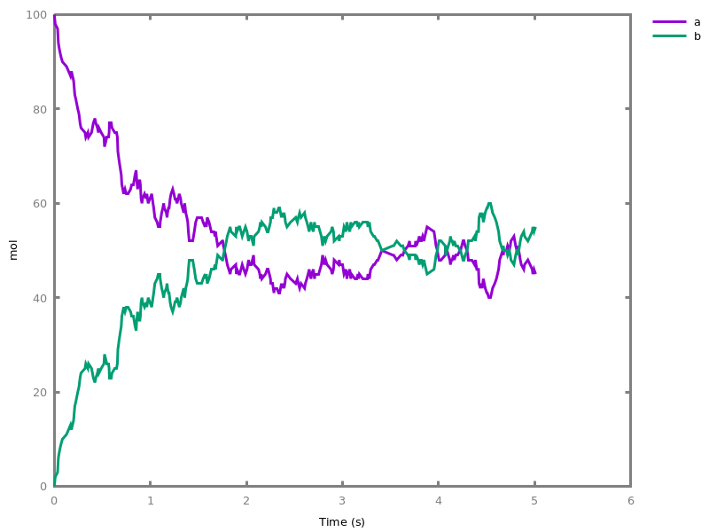
option.sets options globally.Example.biocham:option(time:20, method:bsimp).quit.quits the interpreter.seed(number).For the sake of reproducibility of the results with randomized algorithms, sets the seed of the random number generator to some integer. Note however than the results may still differ on different machines.prolog(Term: name).Just for development purposes, calls a Prolog term written between quotes and prints the result substitution. E.g. when you need to modify the SWI-prolog flags from the toplevel of Biocham: "prolog('set_prolog_flag(stack_limit, 2 000 000 000)')."keep_temporary_files.Switch to a mode where Biocham commands keep the temporary files they generate.delete_temporary_files.Switch to a mode where Biocham commands delete the temporary files they generate. (Default)reset_options.Reset all options to their default values.with_timer(Goal, Time).Execute a given Goal in a given Time (in ms). If no second argument is given, it displays the time taken to execute the command in the standard output.with_timer(Goal).Example.biocham:with_timer(a+b => c).The previous command takes 0.777006 ms
about.lists the version, copyright, license and URL of BiochamPart I: Biochemical Networks
This part describes the syntax of BIOCHAM models of biochemical processes. They are essentially of two forms:- reaction networks (i.e. Feinberg's Chemical Reaction Networks, CRNs, compatible with SBML)
- influence networks (variant of Thomas's regulatory networks, compatible with qualSBML).
Both types of models can be combined and interpreted in a hierarchy of semantics, including the differential semantics (Ordinary Differential Equations), stochastic semantics (Continuous-time Markov Chain), Petri net semantics, and Boolean semantics including several variants defined by options [FMRS18tcbb].Chapter 2
Basic Syntax2.1. Names and arithmetic expressions
The syntax of Biocham is described with formal grammar rules which define new syntactic tokens from primitive tokens such as atom (i.e. string), number, term (e.g. atom(..., ...)).For instance, the syntax of an input or output file is just the syntax of an atom in both cases, but they are distinguished in this manual for documentation purposes:input_file ::= output_file ::= Note that these atoms can enclose with single quotes (') usual UNIX file expansion wildcards like * or ?.The syntax of elementary types in Biocham is the following:concentration ::= time ::= name ::= parameter_name ::= function_prototype ::= object ::= arithmetic_expression ::= condition ::= |true|falseyesno ::= |yes|nolist_molecules.lists all the molecules of the current model.When a molecule is written as compound@location, it represents the given compound as located inside the compartment locationlist_locations.lists all the locations of the current model.list_neighborhood.lists all neighborhood relationships inferred from the model.draw_neighborhood.draws the graph of all neighborhood relationships inferred from the model.2.2. Initial state
list_initial_state.lists the objects which are present (including their initial concentration) and absent from the initial state.clear_initial_state.makes undefined all objects possibly present or absent in the initial state.present({object1, ..., objectn}).Every object in[object1, ..., objectn]is made present in the initial state with initial concentration equal to 1.present({object1, ..., objectn}, concentration).Every object in[object1, ..., objectn]is initialized with the given initialconcentration, which can be a parameter name to indicate that the parameter value will be used. An initial value equal to 0 is equivalent to absent.absent({object1, ..., objectn}).undefined({object1, ..., objectn}).Every object in[object1, ..., objectn]is made possibly present or absent in the initial state. This is the default.initial_state(object1 = concentration1, ..., objectn = concentrationn).Sets the value of initial concentration.make_present_not_absent.makes all objects (appearing in the instances of the current set of rules) which are not declared absent, present in the initial state.make_absent_not_present.makes all objects (appearing in the instances of the current set of rules) which are not declared present, absent in the initial state.2.3. Parameters
parameter(parameter_name1 = arithmetic_expression1,
       ...,
       parameter_namen =
       arithmetic_expressionn).
sets parameter values to numbers or to the result of ground arithmetic expressions (not involving user defined functions or other parameters).list_parameters.shows the values of all known parameters.delete_parameter(parameter_name1, ..., parameter_namen).deletes some parameters2.4. Functions
function(function_prototype1 = arithmetic_expression1,
       ...,
       function_prototypen =
       arithmetic_expressionn).
sets the definition of functions.list_functions.lists all known functions.delete_function(functor1, ..., functorn).deletes some functions. Either arity is given, or all functions with the given functor are deleted.evaluate(Expr: arithmetic_expression).Evaluates an arithmetic expression possibly containing user-defined functions, parameters and molecule names denoting their initial concentration values. Warning: does loop in case of cyclic definitions.Chapter 3
Reaction Networks3.1. Syntax of reactions
(Bio)chemical reaction networks (CRNs) can be described in BIOCHAM by a reaction model, i.e. a finite multiset of directed reaction rules, formed with reactants, products, catalysts and possibly inhibitors, using the syntax defined by the grammar below. Catalysts are molecular species which is both reactant and product in a reaction. They can be noted with an abbreviated syntax between brackets on the arrow. The inhibitors are distinguished in the reactants by following the symbol "⁄" in the left-hand side of the reactions. When not specified, the rate function is by default a mass action law kinetics with rate constant equal to 1. BIOCHAM reaction models are compatible with the Systems Biology Markup Language SBML version 2.reaction ::= rule_name ::= basic_reaction ::= reactants ::= enumeration ::= |_kinetics ::= Example. ,biocham:a+b+c/d,e => f.biocham:_ =[a]=> b.biocham:list_reactions.[0] MA(1) for (a+b+c)/(d,e)=>f [1] MA(1) for a=>a+b
biocham:list_ode.[0] d(b)/dt=a-a*b*c [1] d(f)/dt=a*b*c [2] d(c)/dt= - (a*b*c) [3] d(a)/dt= - (a*b*c) [4] d(d)/dt=0 [5] d(e)/dt=0 [6] init(b=0) [7] init(f=0) [8] init(c=0) [9] init(a=0) [10] init(d=0) [11] init(e=0)
Useful abbreviations for mass action law kinetics (with inhibitors), Michaelis-Menten kinetics, Hill kinetics (with inhibitors).function MA(k) = k * product(S * M in [reactants], M ^ S).function MAI(k) = k * product(S * M in [reactants], M ^ S) / (1 + sum(M in [inhibitors], M)).function MM(Vm, Km) = Vm * single_reactant / (Km + single_reactant) .function Hill(Vm, Km, n) = Vm * single_reactant ^ n / (Km ^ n + single_reactant ^ n) .function HillI(Vm, Km, n) = Vm * single_reactant ^ n / (Km ^ n + single_reactant ^ n + sum(M in [inhibitors], M ^ n)).3.2. Aliases
alias(object1 = ... = objectn).makesObjectsbe alternative names for the same object.biocham:a=>b.biocham:b=>c.biocham:c=>a.biocham:list_reactions.[0] MA(1) for a=>b [1] MA(1) for b=>c [2] MA(1) for c=>a
biocham:alias(a=c).biocham:list_reactions.[0] MA(1) for a=>b [1] MA(1) for b=>a [2] MA(1) for a=>a
canonical(object).makesobjectbe the canonical representant for all its aliases.list_aliases.shows the values of all known aliases.delete_alias(object).makesobjectdistinct from all other objects.3.3. Reaction editor
add_reaction(reaction).adds reaction rules to the current set of reactions. This command is implicit: reaction rules are directly added when reading them.Remark. In Biocham v4, a reaction network is represented by a multiset of reactions. Reactions can thus be added in multiple copies in which case their reaction rates are summed.delete_reaction(reaction).removes one reaction rule from the current set of reactions.delete_reaction_named(name).removes reaction rules by their name from the current set of reactions.delete_reactions.Removes all reaction rules from the current model.delete_reaction_prefixed(Prefix: name).removes all the reaction rules that match a name prefix.merge_reactions(reaction1, reaction2).merges two reaction rules by removing them and replacing them by a new reaction with reactants the sum of reactants, with products the sum of the products, and with kinetics the product of the kinetics (using mass action law kinetics if MA, MAI, MM or Hill kinetics).list_reactions.lists the current set of reaction rules.list_rules.lists the current set of reaction and influence rules.list_reactions_with_species({object1, ..., objectn}).Lists reactions having a reactant, product or inhibitor in the set of molecular speciesObjectset.list_reactions_with_reactant({object1, ..., objectn}).Lists reactions having a reactant in the set of molecular speciesObjectset.list_reactions_with_product({object1, ..., objectn}).Lists reactions having a product in the set of molecular speciesObjectset.list_reactions_with_catalyst({object1, ..., objectn}).Lists reactions with a catalyst (i.e. both reactant and product) in the set of molecular speciesObjectset.list_reactions_with_strict_catalyst({object1, ..., objectn}).Lists reactions with a strict catalyst (i.e. same stoichiometry as reactant and product) in the set of molecular speciesObjectset.list_reactions_with_autocatalyst({object1, ..., objectn}).Lists reactions with an autocatalyst (i.e. different stoichiometry as reactant and product) in the set of molecular speciesObjectset.list_reactions_with_inhibitor({object1, ..., objectn}).Lists reactions with an inhibitor in the set of molecular speciesObjectset.3.4. Reaction graph visualization
up_type ::= |none|present|sourcesDefines if in the drawing of a graph using Graphviz, some species should appear first (i.e. on top of the drawing, or at the left if dran from left to right. The default value ispresent, i.e. draw first the species that are present in the initial state.option(draw_first:present).The bipartite graph of molecular species and reactions can be drawn with the following command.draw_reactions.Draws the reaction graph of the current model. Equivalent toreaction_graph. draw_graph.Example.biocham:load(library:examples/mapk/mapk).biocham:draw_reactions.
reaction_graph.Builds the reaction graph of the current model.Example.biocham:option(draw_first:none,left_to_right:no).biocham:draw_reactions.
Options.
- draw_first: up_type
- Put species of this type at the top of the graph when drawing it.
rule_graph.Builds the rule graph of the current model, i.e. the union of the reaction graph and the influence graph.import_reactions_from_graph.Updates the set of reactions of the current model with the current graph.draw_rules.Draws the reaction graph of the current model. Equivalent torule_graph. draw_graph.The graph is either drawn from left to right (default) or from top to bottom.option(left_to_right:yes).draw_graph.Draws the current graph.Options.
- left_to_right: yesno
- Draws the graph from left to right (default) instead of top to bottom, with species present in the initial state first.
export_graph(output_file).Exports the current graph in a file. The format is chosen from the suffix:.dot,.pdf,.eps,.ps,.pngor.svg– assuming no extension is.dot.3.5. Graph editor
Different graphs can be created from Biocham models and manipulated and more importantly visualized using the third-party Graphviz visualization tool.edgeref ::= new_graph.Creates a new graph.delete_graph(name).Deletes a graph.set_graph_name(name).Sets the name of the current graph.list_graphs.Lists the graph of the current model.select_graph(name).Selects a graphadd_vertex(name1, ..., namen).Adds new vertices to the current graph.delete_vertex(name1, ..., namen).Deletes a set of vertices from the current graph.add_edge(edge1, ..., edgen).Adds the given set of edges to the current graph. The vertices are added if needed.delete_edge(edgeref1, ..., edgerefn).Deletes a set of edges from the current graph.list_edges.Lists the edges of the current graph.list_isolated_vertices.Lists the isolated vertices of the current graph.list_graph_objects.Lists the edges and the isolated vertices of the current graph, and their attributes if any.set_attribute({graph_object1, ..., graph_objectn}, attribute).Adds an attribute to every vertex or edge in the given set. The vertices and the edges are added if needed.place(name1, ..., namen).transition(name1, ..., namen).delete_attribute(graph_object, Attribute: name).Removes an attribute fromgraph_object.list_attributes(graph_object).List the attributes ofgraph_object.Chapter 4
Influence NetworksBIOCHAM models can also be defined by influence systems with forces, possibly mixed to reactions with rates.In the syntax described by the grammar below, one influence rule (either positive "->" or negative "-<") expresses that a conjunction of sources (or their negation after the separator "⁄" for inhibitors) has an influence on a target molecular species. This syntax necessitates to write the Boolean activation (resp. deactivation) functions of the molecular species in Disjunctive Normal Form, i.e. with several positive (resp. negative) influences in which the sources are interpreted by a conjunction [FMRS18tcbb].influence ::= inputs ::= 4.1. Influence editor
add_influence(influence).adds influence rules to the current set of influences. This command is implicit: influence rules can be added directly in influence models.Example. This example shows a positive influence on b with both a positive source, a, and a negative source (i.e. an inhibitor), b. The positive and negative sources have opposite effects on the force of the influence, but do not change the nature of the influence, i.e. the activation of b. This motivates the use of the positive Boolean semantics which simply ignores the inhibitors and the forces. On the other hand, the negative Boolean semantics interprets the inhibitors as negative conditions for the influence. The second influence in this example is added to show the difference between both Boolean dynamics.biocham:parameter(k=1).biocham:present(a,1).biocham:MA(k)/(1+b) for a / b -> b.biocham:list_ode.[0] d(b)/dt=a*k/(1+b) [1] d(a)/dt=0 [2] init(b=0) [3] init(a=1) [4] par(k=1)
biocham:numerical_simulation.biocham:plot.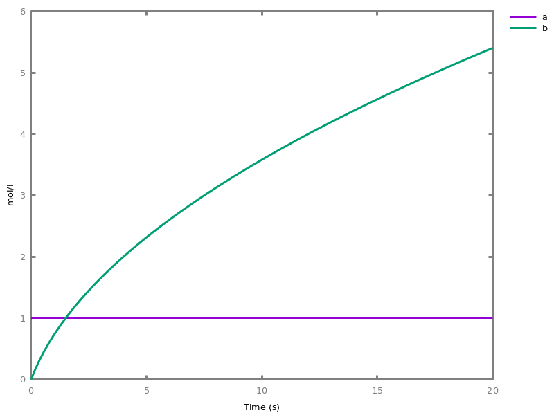
biocham:absent(b). absent(c).biocham:MA(k)/(1+a) for b / a -> c.biocham:option(boolean_semantics:positive).biocham:generate_ctl_not.reachable(stable(a)) reachable(stable(b)) reachable(stable(c)) reachable(steady(not c)) reachable(not b) checkpoint2(a,b) checkpoint2(a,c) checkpoint2(b,c) checkpoint2(not c,b) checkpoint2(not b,c)
biocham:option(boolean_semantics:negative).biocham:generate_ctl_not.reachable(stable(a)) reachable(stable(b)) reachable(stable(not c)) reachable(not b) checkpoint2(a,b) checkpoint2(not c,b)
list_influences.lists the current set of influence rules.influence_model.creates a new influence model by inferring the influences between all molecular objects of the current hybrid modelreaction_model.creates a new reaction model by inferring the reactions between all molecular objects of the current hybrid model4.2. Influence graphs
Biocham can manipulate three notions of influence graph of a model.First, the influence hypergraph of an influence network or a reaction network depicts the structure of the influences between the constituants of a model. It is represented by a bipartite molecule-influence graph.influence_hypergraph.builds the hypergraph of the influence rules of the current model.draw_influence_hypergraph.Draws the hypergraph of the influence rules of the current model. The hypergraph distinguishes each influence. Equivalent toinfluence_hypergraph. draw_graph.Second, the influence graph of a reaction or influence network is a signed directed simple graph between the molecular species. This graph an abstraction defined from the stoichiometry of the reactions, which is equivalent, under general conditions, to the influence graph defined by the signs of the Jacobian matrix of the ODEs [FS08fmsb,FGS15tcs].influence_graph.builds the influence graph between molecular species of the current model without distinguishing between reaction and influence rules.draw_influences.draws the influence graph between molecular species of the current model. Equivalent toinfluence_graph. draw_graph.Example.biocham:load(library:examples/mapk/mapk).biocham:draw_influences. Third, the multistability graph is a multigraph variant of the influence graph in which the influence arcs are labelled by the reactions from which they originate. This labelled graph can be used for checking very efficiently necessary conditions for the existence of oscillations and multiple steady states [BFS18jtb] (
check_multistability/0).option(force_graph:no).multistability_graph.Creates the influence graph of the current model as byinfluence_graph/1but with the arcs labelled with the reactions they originate from. This is used for commandcheck_multistability/0.Options.
- force_graph: yesno
- Force the creation of the graph
export_lemon_graph(output_file).exports the current influence or multistability graph tooutput_filein Lemon graph format (http://lemon.cs.elte.hu/trac/lemon) (adding.lgfextension if needed). Computes the conservation laws of the model (bysearch_conservations/0) in order to do so.Chapter 5
EventsEvents can be used to change some parameter values once a condition gets satisfied. This is useful to implement discrete events in a variety of situations. Events can be used in modelling, for instance for dividing the cell mass by 2 at each division in a model of the cell cycle, or for creating hybrid automata model, which chain different continuous semantics (ODEs). Events can also be intensively used to implement stochastic simulators defined by events, and hybrid differential-stochastic simulators [CFJS15tomacs].add_event(condition, parameter_name1 = arithmetic_expression1, ..., parameter_namen = arithmetic_expressionn).sets up an event that will be fired each time the condition given as first argument goes from false to true. This command is effective in numerical simulations only. Upon firing, the parameters receive new values computed from the expression. The initial values of the parameters are restored after the simulation.Example.biocham:'MA'(k)for a=>b.biocham:parameter(k=1).biocham:add_event(b>0.4,k=0).biocham:present(a).biocham:numerical_simulation(time:2).biocham:plot.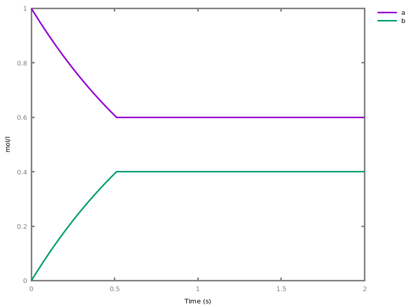
biocham:numerical_simulation(time:2,method:ssa).biocham:plot.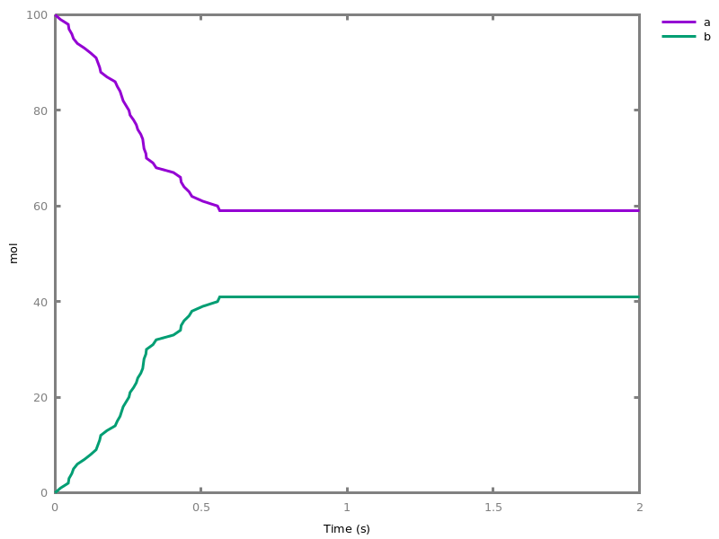 Note that the continuous
numerical_simulation/0engine will attempt to interpolate linear event conditions as per [doi.org/10.1007/3-540-45351-2_19].add_time_event(Expression: arithmetic_expression, parameter_name1 = arithmetic_expression1, ..., parameter_namen = arithmetic_expressionn).Introduce a special kind of event that will be fired when the time reaches the given threshold. They may be used for efficiency reason during numerical integration.list_events.lists all the declared events.delete_events.deletes all the declared events.Chapter 6
Importing and Exporting BIOCHAM Models6.1. Biocham files
load(input_file).acts as the correspondingload_biocham/1⁄load_sbml/1⁄load_model_from_ode/1⁄load_table/1, depending on the file extension (respectively.bc,.xml,.ode,.csv– assuming no extension is.bc). If you need to just import an ode system, useimport_ode/1.Options.
- use_sbml_id: yesno
- Use the sbml_id for the import of all sbml object instead of their names
add(input_file).acts as the correspondingadd_biocham/1⁄add_sbml/1⁄add_model_from_ode/1⁄add_table/1, depending on the file extension (respectively.bc,.xml,.ode,.csv– assuming no extension is.bc).Options.
- use_sbml_id: yesno
- Use the sbml_id for the import of all sbml object instead of their names
load_biocham(input_file).opens a new model, loads the reaction rules and executes the commands (with the file directory as current directory) contained in the given Biocham.bcfile. The suffix.bcis automatically added to the name if such a file exists.add_biocham(input_file).the rules of the given.bcfile are loaded and added to the current set of rules. The commands contained in the file are executed (with the file directory as current directory).export_biocham(output_file).exports the current model into a.bcfile.new_model.opens a new fresh model.new_model(ModelName).opens a new fresh model with a selected name.clear_model.clears the current model.list_models.lists all open models.list_current_models.lists current models.list_model.lists the current Biocham model: reactions, influences, initial state, parameters, events, functions, LTL patterns, options.select_model({ref1, ..., refn}).selects some models.set_model_name(name).changes the current model name.inherits(ref1, ..., refn).makes the current model inherit from the given ancestor models.parametrize.Replace numeric constants in a model by parameters k1, k2,... initialized with their value.check_model.Checks whether the current model is well formed and strict, (see TCS15_FGS).If it is not the case, proposes a witness.check_polynomiality.Check whether the current ODE system is polynomial.correct_model.Improve wellformedness and strictness of a CRN model by removing reactions of null kinetics, splitting reactions that are implicitely reversible in two and adding correct annotation for modifiers.6.2. SBML and SBML-qual files
option(use_sbml_id:no).load_sbml(input_file).acts asload_biocham/1, this import the species, reactions, parameters, compartments, events and initial states from the provided SBML .xml file. By default, we use the sbml Names of the species as biocham identifier. When this leads to naming conflicts, we suffix these names with the sbml Id. The option use_sbml_id (default: no) allows to bypass this naming and simply use the id as identifier. Rq: Notes and annotations are imported but are not accessible for the user.Options.
- use_sbml_id: yesno
- Use the sbml_id for the import of all sbml object instead of their names
add_sbml(input_file).acts asadd_biocham/1but importing reactions, parameters and initial state (and only that!) from an SBML .xml file.option(output_to_library:no).download_curated_biomodel(Id: integer).Downloads to the current directory the SBML file for the corresponding (curated) biomodel with numeric IDId(e.g. "5").Options.
- output_to_library: yesno
- outputs to the library⁄biomodels subfolder
export_sbml(output_file).exports the current model into an SBML.xmlfile.load_qual(input_file).acts asload_biocham/1but importing influences and initial state (and only that!) from an SBML3qual .sbml file.add_qual(input_file).acts asadd_biocham/1but importing influences and initial state (and only that!) from an SBML3qual .sbml file.load_ginml(input_file).acts asload_biocham/1but importing influences from a GINsim .ginml file.add_ginml(input_file).acts asadd_biocham/1but importing influences from a GINsim .ginml file.6.3. Ordinary Differential Equation Models
Biocham can also manipulate ODE systems, import and export ODE systems in XPP syntax, and export them in LaTeX.Remark. XPP format has restrictions on names and does not distinguish between upper case and lower case letters. For that reason, and in order to avoid misinterpretations, when an XPP file is imported, all names are read in lower case.The ODE simulation of a Biocham model proceeds by creating an ODE system if there is none, and deleting it after the simulation.It is worth noting that if there is an ODE system present, it is the current ODE system that is simulated, not the Biocham model.Biocham can also infer an equivalent reaction network or influence network from the ODEs [FGS15tcs]. This is useful for importing MatLab models in SBML, and using Biocham analyzers on ODE models.ode ::= oderef ::= Listing ODEs
list_ode.returns the set of ordinary differential equations and initial concentrations (one line per molecule) associated to the current model or ODE system.Example.biocham:a=>b.biocham:list_ode.[0] d(b)/dt=a [1] d(a)/dt= -a [2] init(b=0) [3] init(a=0)
Exporting ODEsexport_ode(output_file).exports the ODE system of the current model.export_ode_as_latex(output_file).exports the ODE system of the current model as LaTeX code.Inferring reaction or influence networks from an ODE file
Example.biocham:parameter(k=10).biocham:MA(k) for 2*a + b => 3*c.biocham:list_ode.[0] d(c)/dt=3*a^2*b*k [1] d(a)/dt= - (2*a^2*b*k) [2] d(b)/dt= - (a^2*b*k) [3] init(c=0) [4] init(a=0) [5] init(b=0) [6] par(k=10)
biocham:export_ode('test2.ode').biocham:load_reactions_from_ode('test2.ode').biocham:list_model.MA(k) for b+2*a=>3*c. parameter( k = 10 ).
biocham:load_influences_from_ode('test2.ode').biocham:list_model.3*(a^2*b*k) for a,b -> c. 1*(a^2*b*k) for a,b -< b. 2*(a^2*b*k) for a,b -< a. initial_state(c=0). initial_state(a=0). initial_state(b=0). parameter( k = 10 ).
biocham:list_ode.[0] d(a)/dt= - (2*a^2*b*k) [1] d(b)/dt= - (a^2*b*k) [2] d(c)/dt=3*a^2*b*k [3] init(a=0) [4] init(b=0) [5] init(c=0) [6] par(k=10)
option(import_reactions_with_inhibitors:yes).load_reactions_from_ode(input_file).infers a set of reactions equivalent to an ODE system, and loads it asload_biocham/1.Options.
- import_reactions_with_inhibitors: yesno
- Add inhibitors when inferring reactions (default yes).
add_reactions_from_ode(input_file).infers a set of reactions equivalent to an ODE system, and adds it to the current model asadd_biocham/1.Options.
load_influences_from_ode(input_file).infers a set of influences equivalent to an ODE system, and loads it asload_biocham/1.add_influences_from_ode(input_file).infers a set of influences equivalent to an ODE system, and adds it to the current model asadd_biocham/1.ODE systems
option(second_order_closure:no).ode_system.builds the set of ODEs of the current model.Options.
- second_order_closure: yesno
- Compute (normal) second order moment closure ODEs. Introduce covariance variables and functions to visualize plus⁄minus standard deviation
import_ode(input_file).imports a set of ODEs.new_ode_system.creates an ODE system.delete_ode_system(name).deletes an ODE system.clear_ode_systems.Remove all existing ODE systems.set_ode_system_name(name).sets the name of the current ODE system.list_ode_systems.lists the ODE systems of the current model.select_ode_system(name).selects an ODE systemadd_ode(ode1, ..., oden).If there is a current ODE system, adds the given set of ODEs to it. If there is no current ODE system, infers reactions equivalent to the given set of ODEs.delete_ode(oderef1, ..., oderefn).removes the given set of ODEs from the current ODE system.init(name1 = arithmetic_expression1, ..., namen = arithmetic_expressionn).sets the initial value of a variable in the current set of ODEs.option(infer_hidden_molecules:no).add_reactions_from_ode_system.adds a set of reactions equivalent to the current ODE system.Options.
- import_reactions_with_inhibitors: yesno
- Add inhibitors when inferring reactions.
add_influences_from_ode_system.adds a set of influences equivalent to the current ODE system.load_reactions_from_ode_system.Replaces the current reactions with those fromadd_reactions_from_ode_system/0.Options.
load_influences_from_ode_system.Replaces the current reactions with those fromadd_influences_from_ode_system/0.remove_fraction.Remove the rational fraction in the current ODE system by multiplying the derivative by the GCD. WARNING: the resulting ODE system is NOT equivalent to the starting one.infer_hidden_molecules.Tries to infer hidden molecules eliminated by linear invariants.ode_parameter(name1 = number1, ..., namen = numbern).sets the value of a parameter in the current set of ODEs.ode_function(name1 = arithmetic_expression1, ..., namen = arithmetic_expressionn).defines a (parameterless) function in the current set of ODEs.load_model_from_ode(input_file).Clean the current model and import the .ode⁄.xpp file then calladd_model_from_ode/1.add_model_from_ode(input_file).Import the .ode⁄.xpp file and infer the corresponding reactions or influences system.export_xpp(output_file).Exports the ODE system of the current model as an XPP file.read_xpp(input_file).Imports an ODE system from an XPP file.Part II: Qualitative Analysis and Synthesis
Chapter 7
Static Analyses7.1. Graph properties
Analysis of some graph properties of the current model.pathway(object1, object2).Gives one reaction pathway fromobject1toobject2if one exists in the directed reaction graph of the current model (for more complex queries, see next section on Computation Tree Logic model-checking).list_input_species.Lists the molecular species that are neither a reaction product apart from strict catalysts, nor the target of an influence rule, in the curent model. Reactants that are not catalysts, and strict catalysts, i.e. catalysts with same stoichiometry in left-hand and right side of reactions, are allowed as inputs.list_strict_input_species.Lists the molecular species that are strict catalysts, i.e. neither a strict product, nor strict reactant, nor the target of an influence rule in the curent model.list_source_species.Lists the molecular species that are neither a reaction product nor the target of an influence rule in the curent model.list_sink_species.Lists the molecular species that are neither a reactant nor a positive source of an influence rule in the curent model.7.2. Dimensional analysis
unit_type ::= |time|volume|substanceset_units(Type: unit_type, Unit: name).Set the default units for the given type (time, volume or substance) in the current model.list_units.Lists the default units of the current model.Dimensional analysis infers dimensions for model parameters and checks their consistency. In Biocham, only time and volume dimensions are considered. The dimension of a molecular concentration is volume$^{-1}$. Warning: numbers have no dimension so kinetic parameters should be used in kinetic expressions instead of directly numbers.list_dimensions.Infers the time and volume dimensions of all parameters according to ODEs. An error is raised if some parameters appear in expressions with inconsistent dimensions. This can happen in a model if some multiplicative parameter with value equal to 1 is omitted for example.Example.biocham:MM(v, k) for A => B.biocham:parameter(k = 2, v = 3).biocham:list_dimensions.v has dimension time^(-1).volume^(-1) k has dimension time^(0).volume^(-1)
set_dimension(P: parameter_name, U: number, V: number).Declare dimension time^U. volume^Vfor parameterPclear_dimensions.Clear all declared dimensionsclear_dimension(P: parameter_name).Clear declared dimension for parameterP7.3. Conservation laws and invariants
Petri Net Place-invariants provide linear conservation laws for the differential semantics of a reaction network. They can be verified or computed with the commands below. Note that such invariants are useful information but it may be not a good idea to use them to reduce the dimensionality of the system since it may introduce numerical instabilities.add_conservation(Conservation: solution).declares a new mass conservation law for all molecules given with the corresponding weight inConservation. During a numerical simulation, one of those variables will be eliminated thanks to this conservation law. Be careful if you declare conservation laws and then plot the result of a previous simulation, the caption might not be correct. When added, the conservation law will be checked against the reactions (i.e. purely from stoichiometry), if that fails against the kinetics. Since these checks are not complete, even a failure will be accepted with a warning.delete_conservation(Conservation: solution).removes the given mass conservation law.delete_conservations.removes all mass conservation laws.list_conservations.prints out all the mass conservation laws.check_conservations.checks all conservation laws against reactions, and if necessary kinetics (see alsoadd_conservation/1).option(conservation_size:4).search_conservations.computes and displays the P-invariants of the network up to the maximal size given by the option conservation_size and defaulting to 4. Such P-invariants are particular mass conservation laws that are independent from the kinetics.Options.
- conservation_size: integer
- Set the maximal stoichiometric size for a P-invariant.
search_efms.computes and displays the T-invariants of the network up to the maximal flux given by the option conservation_size and defaulting to 4. Such T-invariants can be seen as a way to compute Extreme Rays of the cone of Elementary Flux Modes.Options.
- conservation_size: integer
- Set the maximal stoichiometric size for a P-invariant.
7.4. Detecting model reductions
This section describes commands to detect model reduction relationships between reaction models based solely on the structure of their reaction graph [GSF10bi]. The commands below check the existence of a subgraph epimorphism (SEPI) [GFS14dam], i.e. a graph reduction from one graph to a second graph, obtained by deleting and⁄or merging species and⁄or reactions. A SAT solver is used to solve this NP-complete problem.extremal_sepi ::= |Search standard reduction.no|Search reduction that minimises bottom (i.e., the number of deletions).minimal_deletion|Search reduction that maximises bottom (i.e., the number of deletions).maximal_deletionmerge_restriction ::= |Search standard reduction.no|Search reduction with local two-neighbour restriction (cf. report chapter 5).neighbours|Search reduction while forbidding to merge species together.not_species|Search reduction with old two-neighbour restriction (prior to 2019).oldoption(mapping_restriction:[]).option(merge_restriction:no).option(timeout:180).option(all_reductions:no).option(distinct_species:no).option(max_nb_reductions:200).option(extremal_sepi:no).option(stats:no).option(show_support:no).search_reduction(FileName1: input_file, FileName2: input_file).checks whether there exists one model reduction from a first Biocham model to a second model, and returns the first model reduction found, as a description of a graph morphism (SEPI) from the reaction graph of the first model to the second. Optionally, a partial mapping of the form ['label1' -> 'label2', 'label3' -> 'deleted'] can be given to restrict the search to reductions satisfying this mapping of molecular names. Another option restricts the merge operation to nodes sharing at least one neigbour in the reaction graph. A timeout option can be given in seconds (default is 180s). Note that the files FileName1 and FileName2 will be loaded, therefore any previous model will be overwritten and some biocham commands might be executed.Options.
- mapping_restriction: [basic_influence1, ..., basic_influencen]
- enforce the given mappings in the SEPI
- merge_restriction: merge_restriction
- restrict merges according to some criterion
- timeout: number
- timeout for the (Max)SAT solver
- all_reductions: yesno
- specifies if solver is looking for all SEPI reductions or not
- distinct_species: yesno
- specifies if solver is listing only SEPIs with distinct species (cf. report section 6.6)
- max_nb_reductions: number
- limits the number of SEPI reductions the solver is looking for
- extremal_sepi: extremal_sepi
- defines the type of reduction searched (cf. report chapter 3)
- show_support: yesno
- determine if the printing describe the SEPI or only its support.
- stats: yesno
- display computation time
Example. Detecting Michaelis-Menten reductions:biocham:load(library:examples/sepi/MM1.bc).biocham:list_model.MA(1) for E+S=>ES. MA(1) for ES=>E+S. MA(1) for ES=>E+P.
biocham:load(library:examples/sepi/MM2.bc).biocham:list_model.MA(1) for A+B=>A+C.
biocham:search_reduction(library:examples/sepi/MM2.bc, library:examples/sepi/MM1.bc).no sepi found
biocham:search_reduction(library:examples/sepi/MM1.bc, library:examples/sepi/MM2.bc, mapping_restriction: [E->A]).sepi E -> A S -> B ES -> deleted P -> C {E+S => ES} -> {A+B => A+C} {ES => E+S} -> deleted {ES => E+P} -> {A+B => A+C} Number of reductions: 17.5. Pattern reduction
This section describes commands to rewrite a reaction graph by reducing some specified patterns (for example Michaelis-Menten patterns). The idea behind this function is to use graph rewriting before searching SEPIs (with the commandsearch_reduction/2. It is also possible to expand reduced Michaelis-Menten patterns, in order to exhibit the intermediary step of reversible complexation enzyme-substrate.option(michaelis_menten:yes).option(r_1:yes).option(r_2:no).option(ep:no).option(enzyme:yes).option(hill_reaction:no).option(partial_hill_reaction:no).option(double_michaelis_menten:no).option(michaelis_menten_expansion:no).yesnomaybe ::= |Value yes.yes|Value no.no|Value maybe.maybepattern_reduction(Input_file: input_file, Output_file: input_file).The patterns to be searched into the input graph (the graph associated to the Biocham model given asInput_file) are specified by the options. For a pattern, being found into a graph means that there is a subgraph isomorphism from the graph to the pattern and that only the vertices sent to the image vertices enzyme, substrate, product can have edges with other vertices in the graph (for example it constrains the complex not to intervene in any other reaction). The number of found patterns is printed in the terminal. In the output model (written in a new file .bc, with name specified by the user asOutput_file), all occurrences of these patterns are reduced to the one-reaction Michaelis-Menten pattern, with a double-arrow from the enzyme. The michaelis_menten_expansion option has the opposite effect to expand reduced Michaelis-Menten patternsOptions.
- michaelis_menten: yesno
- specifies if reducing Michaelis-Menten patterns
- r_1: yesnomaybe
- R-1 reaction (from the commplex ES to enzyme E and substrate S) in the searched Michaelis-Menten pattern
- r_2: yesnomaybe
- R-2 reaction (from the product P and enzyme E to the complex EP or ES) in the searched Michaelis-Menten pattern
- ep: yesnomaybe
- irreversible reaction from the complex ES to the complex EP in the searched Michaelis-Menten pattern
- hill_reaction: yesno
- specifies if reducing Hill patterns
- partial_hill_reaction: yesno
- specifies if reducing partial Hill patterns
- double_michaelis_menten: yesno
- specifies if reducing double Michaelis-Menten
- enzyme: yesno
- specifies if the reduced Michaelis-Menten pattern (that will appear in the output graph) is with enzyme or no
- michaelis_menten_expansion: yesno
- expansion of Michaelis-Menten patterns (form the reduced form with enzyme to form with complex ES and reaction R-1), should be used with option michaelis_menten:no to avoid confusion
Example. Example of reduction of a Michaelis-Menten pattern with reactions R-1, R-2 and complex EP. Input graph :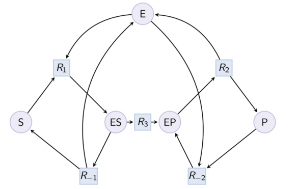
biocham:load(library:examples/sepi/MM_variants/MM_ESP.bc).biocham:option(michaelis_menten:yes).biocham:option(r_1:maybe,r_2:maybe,ep:maybe).biocham:pattern_reduction(library:examples/sepi/MM_variants/MM_ESP.bc, MM_ESP_reduced.bc).Number of Michaelis Menten patterns: 1
biocham:load(MM_ESP_reduced.bc).Output graph (reduced Michaelis-Menten pattern) :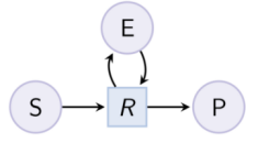 Example. Hill pattern (can be reduced with option hill_reaction) :
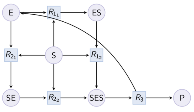 Example. Partial Hill pattern (can be reduced with option partial_hill_reaction) :
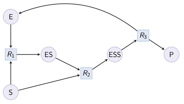 Example. Double Michaelis-Menten pattern (can be reduced with option double_michaelis_menten) :
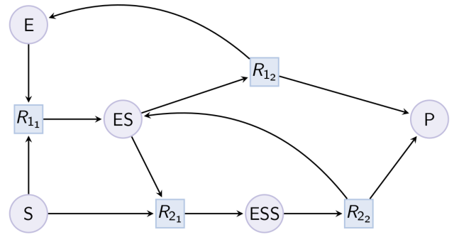 Example. Example of expansion of reduced Michaelis-Menten in a MAPK cascade.
biocham:load(library:examples/sepi/mapk0.bc).biocham:draw_reactions.
biocham:option(michaelis_menten:no).biocham:option(michaelis_menten_expansion:yes).biocham:pattern_reduction(library:examples/sepi/mapk0.bc, mapk0_expanded.bc).Number of Michaelis Menten patterns: 2
biocham:load(mapk0_expanded.bc).biocham:draw_reactions.
7.6. Tropical algebra equilibrations
Tropical algebra can be used to reason about orders of magnitude of molecular concentrations, kinetic parameters and reactions rates.While steady state analysis consists in finding the roots of the differential functions associated to all or some molecular species in a CRN, tropical equilibration consists in finding when the positive and negative preponderant terms of the differential functions have the same order of magnitude (i.e. same integer logarithm).The solutions to tropical equilibration problems provide candidates for regimes exhibiting fast-slow dynamics leading to model reductions based on quasi-steady states or reactions in quasi-equilibrium [SFR14amb].option(tropical_epsilon:0.1).option(tropical_max_degree:3).option(tropical_ignore:{}).option(tropical_denominator:0).option(tropical_single_solution:no).tropicalize.Try to solve a tropical equilibration problem.Example.biocham:load(library:examples/cell_cycle/Tyson_1991.bc).biocham:tropicalize(tropical_max_degree: 2).Cdc2+Cdc2-Cyclin~{p1,p2}+Cdc2-Cyclin~{p1}+Cdc2~{p1} 1 complex invariant(s) found a complete equilibration leading to the rescaling: Cdc2' = ε^(- 2) * Cdc2 Cdc2~{p1}' = Cdc2~{p1} Cyclin' = ε^(- 4) * Cyclin Cdc2-Cyclin~{p1,p2}' = Cdc2-Cyclin~{p1,p2} Cdc2-Cyclin~{p1}' = ε^(- 2) * Cdc2-Cyclin~{p1} Cyclin~{p1}' = ε^(- 2) * Cyclin~{p1} found a complete equilibration leading to the rescaling: Cdc2' = ε^(- 3) * Cdc2 Cdc2~{p1}' = ε^(- 1) * Cdc2~{p1} Cyclin' = ε^(- 3) * Cyclin Cdc2-Cyclin~{p1,p2}' = Cdc2-Cyclin~{p1,p2} Cdc2-Cyclin~{p1}' = ε^(- 2) * Cdc2-Cyclin~{p1} Cyclin~{p1}' = ε^(- 2) * Cyclin~{p1} found a complete equilibration leading to the rescaling: Cdc2' = ε^(- 4) * Cdc2 Cdc2~{p1}' = ε^(- 2) * Cdc2~{p1} Cyclin' = ε^(- 2) * Cyclin Cdc2-Cyclin~{p1,p2}' = Cdc2-Cyclin~{p1,p2} Cdc2-Cyclin~{p1}' = ε^(- 2) * Cdc2-Cyclin~{p1} Cyclin~{p1}' = ε^(- 2) * Cyclin~{p1} No (more) complete equilibrationOptions.
- tropical_epsilon: number
- Used for computing degrees (must be < 1)
- tropical_max_degree: number
- Max absolute value of the degree in epsilon as a power of 2
- tropical_ignore: {object1, ..., objectn}
- set of species to ignore for equilibration ({} to ignore none, {-1} to ignore all unbalanced)
- tropical_denominator: number
- Look for solutions that are integers⁄(tropical_denominator+1)
- tropical_single_solution: yesno
- Stop after finding one solution
- stats: yesno
- display computation time
7.7. Multistability analysis
The existence of oscillations and multiple non-degenerate steady states in the differential dynamics of a reaction or influence model can be checked very efficiently by checking necessary conditions for those properties in the multistability graph of the model (seemultistability_graph/0), namely the existence of respectively negative and positive circuits in that graph [BFS18jtb]. Some more computationally expensive conditions are optional.option(test_permutations:no).option(test_transpositions:no).check_multistability.Checks the possibility of multistability in the continuous semantics of the current model. This commands checks a necessary condition for the existence of multiple non-degenerate (i.e. with no variable equal to 0) steady states.Options.
Example.biocham:load("library:biomodels/BIOMD0000000040.xml").biocham:multistability_graph.biocham:draw_graph(left_to_right:yes).
biocham:check_multistability.There may be non-degenerate multistationarity, positive circuit detected.
biocham:check_multistability(test_transpositions:yes).There may be non-degenerate multistationarity, positive circuit detected.
check_oscillations.Checks a necessary condition for the periodic behaviour of the current model.7.8. Rate independence
Under the condition that a CRN is well-formed (i.e. the of species occurring in the rate of a reaction is the set of its reactants, catalysts and inhibitors [FGS15tcs], Biocham can check sufficient conditions that ensure that the outputs of a CRN are independent of the reaction rates [DFS20cmsb].test_rate_independence.Tests graphical sufficient conditions for rate independence of the current model for all output species (assuming well-formed kinetics).test_rate_independence_invariants.Tests invariant sufficient conditions for rate independence of the current model for all output species (assuming well-formed kinetics).7.9. Mean stochastic behavior
Biocham can check sufficient conditions to ensure that, for some molecular species of the current reaction model, the mean stochastic trace is given by the ODE simulation trace, at all time points, and for any conversion factor (i.e. with small molecule numbers, unlike Kurtz's limit theorem). The command returns the list of molecular species for which that property is guaranteed to hold. The condition basically checks that those species are produced by reactions with mass action law kinetics and that polymolecular reactions are restricted to catalytic synthesis reactions with disjoint sets of ancestor species.test_stochastic_mean_ode.Lists the molecular species of the current reaction model for which the ODE simulation trace is guaranteed to be equal to the mean stochastic trace at all time points, for any conversion factor. This is always the case of the strict input species (seelist_strict_input_species/0) which are listed apart.Chapter 8
Boolean Dynamics, Verification and Synthesis8.1. Attractors in the ground Boolean state transition graph
The following commands refer to the Boolean dynamics of a BIOCHAM model, possibly combining reaction rules and influence rules. The Boolean semantics can be either positive (i.e. without negation, the inhibitors are ignored) or negative (the inhibitors of a reaction or an influence are interpreted as negative conditions) [FMSR16cmsb]. The notion of Boolean states considered in this first section is the one of complete ground states defined by the presence or absence of each molecular species, unlike the notion of symbolic representation of partial states represented by Boolean constraints and considered in the following sections.list_stable_states.lists stable steady ground Boolean states of the ground state transition graph corresponding to the Boolean semantics of the current model.Options.
- boolean_semantics: boolean_semantics
- Use positive or negative boolean semantics for inhibitors.
- boolean_state_display: boolean_state_display
- choice of display of the boolean states.
list_tscc_candidates.lists possible representative states of Terminal Strongly Connected Components (TSCC) of the ground state transition graph corresponding to the positive semantics of the current model.Options.
- boolean_state_display: boolean_state_display
- choice of display of the boolean states.
8.2. Temporal logic properties of the symbolic Boolean state transition graph
The Computation Tree Logic CTL can be used to express qualitative properties of the Boolean dynamics of BIOCHAM model in a given (set of) initial states [CCDFS04tcs]. CTL extends propositional logic, used to represent set of states symbolically by Boolean constraints, with modal operators, used to specify where (E: on some path, A: on all paths) and when (X: next state, F: finally at some future state, G: globally on all states, U: until a second formula is true, R: release) a formula is true. As in any logic, these modalities can be combined with logical connectives and imbricated, with the only restriction that a temporal operator must be immediately preceded by a path quantifier, e.g.EF(AG(p))expresses the reachability of a stable set of states where proteinpwill always remain present.It is worth noting that in this setting, a propositional formula provides a symbolic representation for a set of ground Boolean states, also called a partial state, or just a state by abuse of notation when there is no ambiguity with the ground Boolean states considered in the previous Section. CTL is well suited to analyze attractors, their reachability and transient properties [TFFT16bi]. It is worth noting that reachability properties in temporal logics are relative to a given set of initial states, they are purely factual and not necessarily causal.The syntax of CTL formulas, plus some useful abbreviations, are defined by the following grammar:ctl ::= |current_specreachable(f) is a shorthand for EF(f)mustreach(f) is a shorthand for AF(f)steady(f) is a shorthand for EG(f)stable(f) is a shorthand for AG(f)checkpoint(f, g) is a shorthand for not EU(not f, g)). Note that such a factual property does not imply any causality relationship from f to g.checkpoint2(f, g) is a shorthand for not(g)⁄\ EF(g)⁄\checkpoint(f,g)oscil2(f) is a shorthand for EU(not(f), f ⁄\ EU(f, not(f) ⁄\ EU(not(f), f))) which is true if f has at least two peaks on one pathoscil3(f) is a shorthand for EU(not(f), f ⁄\ EU(f, not(f) ⁄\ EU(not(f), f ⁄\ EU(f, not(f) ⁄\ EU(not(f), f))))) which is true if f has at least three peaks on one pathoscil(f) is a shorthand for oscil3(f) ⁄\ EG(EF(f) ⁄\ EF(not f)) which is a necessary (not sufficient) condition for infinite oscillations in CTLThe qualitative behavior of a network can be specified by a set of CTL formulas using the following commands:list_ctl.Prints out all formulae from the current CTL specification.expand_ctl(Formula: ctl).shows the expansion in CTL of a formula with patterns.add_ctl(Formula: ctl).Adds a CTL formula to the currently declared CTL specification.delete_ctl(Formula: ctl).Removes a CTL formula to the currently declared CTL specification.clear_ctl.Removes all formulae from the current CTL specification.The set of CTL formulas of some simple form that are true in the current set of initial states can also be automatically generated as a specification of the network using the following commands.generate_ctl(Formula: ctl).adds to the CTL specification all the CTL formulas that are true, not subsumed by another CTL formula in the specification, and that match the argument formula in which the names that are not molecules are treated as wildcards and replaced by distinct molecules of the network. This command is a variant with subsumption test ofadd_ctlif all names match network molecule names, otherwise it enumerates all m^v instances (where m is the number of molecules and v the number of wildcards in the formula).Options.
- boolean_initial_states: boolean_initial_states
- specifies whether the truth value of a formula is for all or some completion of the initial states (present⁄absent⁄undefined).
generate_ctl.adds to the CTL specification all reachable stable, reachable steady, reachable, checkpoint2, and oscil formulas on all molecules (using this order of enumeration for performing subsumption checks).generate_ctl_not.adds to the CTL specification all reachable stable , reachable stable not, reachable steady, reachable steady not, reachable, reachable not, checkpoint2, and oscil formulas on all molecules.cleanup_ctl.cleans up the CTL specification by removing redundant formulae such as reachable(steady(A)) if reachable(stable(A)) is true, etc.Example.biocham:a=>b.biocham:b=>c.biocham:c=>d.biocham:present(b).biocham:make_absent_not_present.biocham:generate_ctl(checkpoint2(x,d)).checkpoint2(b,d) checkpoint2(c,d)
biocham:generate_ctl_not.reachable(stable(d)) reachable(stable(not a)) reachable(stable(not b)) reachable(stable(not c)) reachable(steady(b)) reachable(steady(c)) reachable(steady(not d)) checkpoint2(b,c) checkpoint2(b,d) checkpoint2(c,d) checkpoint2(not a,c) checkpoint2(not d,c) checkpoint2(not a,d) checkpoint2(not c,d) checkpoint2(not a,not b) checkpoint2(not c,not b) checkpoint2(not d,not b) oscil(c)
8.3. Verification of CTL and LTL formulae
CTL properties can be efficiently verified with model-checkers. Biocham uses the NuSMV model checker [nusmv] for which the following options can be specified:boolean_semantics ::= |positive|negativeThe default value isnegativeoption(boolean_semantics:negative).The negative Boolean semantics interpret reaction inhibitors with a negation in the condition. The positive Boolean semantics ignore reaction inhibitors.boolean_initial_states ::= |all|some|all_then_some|presentThe default value isall. The valueall_then_sometries for all initial states, and if that fails, for some. The valuepresenttreats undetermined species as absent.boolean_state_display ::= |present|table|vectorDisplay boolean states as apresentcommand. (default), or a TAB separated table of TRUE⁄FALSE values, or an association-list with 0⁄1 values.option(boolean_initial_states:all).CTL formulae can be checked in all or some initial states.option(boolean_trace:no).Display either a Boolean trace proving the formula in some initial state, or a counter example initial state falsifying the formula (default value is no trace).option(nusmv_topological_order:no).Ordering of variables for the NuSMV model-checker.option(query:current_spec).option(boolean_state_display:present).check_ctl.evaluates the current CTL specification (i.e., the conjunction of all formulae of the current specification) or the content of optionqueryon the current model by calling the NuSMV model-checker. As is usual in Model-Checking, the query is evaluated for all possible initial states (Aiin Biocham v3). This can be changed via theboolean_initial_statesoption.Options.
- query: ctl
- Query to evaluate instead of the current CTL specification.
- boolean_initial_states: boolean_initial_states
- specifies whether the truth value of a formula is for all or some completion of the initial states (present⁄absent⁄undefined).
- boolean_trace: yesno
- shows a proof trace or a counter example initial state if available (default value is "no").
- boolean_semantics: boolean_semantics
- choice of positive⁄negative boolean semantics (positive: reaction inhibitors are ignored; negative: the presence of one reaction inhibitor prevents the reaction to proceed.
- nusmv_topological_order: yesno
- tells NuSMV to keep the order of the variables of the BIOCHAM model for building its internal Binary Decision Diagram.
- boolean_state_display: boolean_state_display
- choice of display of the boolean states.
Example.biocham:present(a).biocham:absent(b).biocham:a=>b.biocham:a+b=>a.biocham:check_ctl(query: EX(not(a) \/ EG(not(b))), boolean_trace:yes).EX(not a\/EG(not b)) is true
biocham:check_ctl(query: EG(not(b)), boolean_trace:yes).Trace: present({a}). EG(not b) is falsebiocham:check_ctl(query:reachable(b),boolean_trace:yes).reachable(b) is true
biocham:generate_ctl.reachable(stable(b)) reachable(steady(a)) checkpoint2(a,b) oscil(b)
biocham:check_ctl.current_spec is true
A Linear Time Logic (LTL) formula contains no path quantifier. The syntax of LTL formulae is given in the next chapter for the more general setting of First-Order LTL (FO-LTL) formulae with numerical constraints. Here a boolean LTL formula is true if it is satisfied by all paths and all boolean initial states. This can be changed by double negation with the optionboolean_initial_states: someto verify that there exists an initial state and a path satisfying the formula. Unlike CTL, the path quantifier cannot be decoupled from the quantifier on the initial state.check_ltl(Query: foltl).evaluates the given boolean LTL specification on the current model by calling the NuSMV model-checker in Bounded Model-Checking mode.Options.
- boolean_initial_states: boolean_initial_states
- specifies whether the truth value of a LTL formula is for all or some completion of the initial states (present⁄absent⁄undefined) and for all or some paths.
- boolean_trace: yesno
- shows a proof trace or a counter example initial state if available (default value is "no").
- boolean_semantics: boolean_semantics
- Use positive or negative boolean semantics for inhibitors.
- boolean_state_display: boolean_state_display
- choice of display of the boolean states.
Example.biocham:present(a).biocham:absent(b).biocham:a=>b.biocham:a+b=>c.biocham:check_ltl(reachable(c), boolean_trace:yes).Trace: present({a}). present({b}). present({b}). Reactions used for that path: MA(1)for a=>b reachable(c) is falsebiocham:check_ltl(reachable(c), boolean_initial_states: some, boolean_trace:yes).Trace: present({a, c}). reachable(c) is trueexport_nusmv(output_file).exports the current Biocham set of reactions and initial state in an SMV.smvfile.Options.
- boolean_semantics: boolean_semantics
- Use positive or negative boolean semantics for inhibitors.
8.4. Model reduction from CTL specification
This section describes commands to reduce a reaction model by deleting species and reactions, while preserving a CTL specification of the behaviour.reduce_model(Query: ctl).Deletes reactions as long as the specification of the behavior given by a CTL formula passed as argument remains satisfied in the current initial state.reduce_model.Same as above using the current CTL specification of the behavior.Example.biocham:a=>b.biocham:b=>c.biocham:c=>d.biocham:present(b).biocham:make_absent_not_present.biocham:generate_ctl.reachable(stable(d)) reachable(steady(b)) reachable(steady(c)) checkpoint2(b,c) checkpoint2(b,d) checkpoint2(c,d) oscil(c)
biocham:reduce_model.removed: MA(1) for a=>b
Example. Reduction of the MAPK model with respect to the output reachability property only: all dephosphorylation reactions can be removed, resulting in a different bifurcation diagram with full memory effect.biocham:load('library:examples/mapk/mapk.bc').biocham:reduce_model(reachable('MAPK~{p1,p2}')).removed: MA(1) for 'RAF-RAFK'=>RAF+RAFK MA(1) for RAFPH+'RAF~{p1}'=>'RAF~{p1}-RAFPH' MA(1) for 'RAF~{p1}-RAFPH'=>RAFPH+'RAF~{p1}' MA(1) for 'MEK-RAF~{p1}'=>MEK+'RAF~{p1}' MA(1) for 'MEK~{p1}-RAF~{p1}'=>'MEK~{p1}'+'RAF~{p1}' MA(1) for MEKPH+'MEK~{p1}'=>'MEK~{p1}-MEKPH' MA(1) for 'MEK~{p1}-MEKPH'=>MEKPH+'MEK~{p1}' MA(1) for MEKPH+'MEK~{p1,p2}'=>'MEK~{p1,p2}-MEKPH' MA(1) for 'MEK~{p1,p2}-MEKPH'=>MEKPH+'MEK~{p1,p2}' MA(1) for 'MAPK-MEK~{p1,p2}'=>MAPK+'MEK~{p1,p2}' MA(1) for 'MAPK~{p1}-MEK~{p1,p2}'=>'MAPK~{p1}'+'MEK~{p1,p2}' MA(1) for MAPKPH+'MAPK~{p1}'=>'MAPK~{p1}-MAPKPH' MA(1) for 'MAPK~{p1}-MAPKPH'=>MAPKPH+'MAPK~{p1}' MA(1) for MAPKPH+'MAPK~{p1,p2}'=>'MAPK~{p1,p2}-MAPKPH' MA(1) for 'MAPK~{p1,p2}-MAPKPH'=>MAPKPH+'MAPK~{p1,p2}' MA(1) for 'RAF~{p1}-RAFPH'=>RAF+RAFPH MA(1) for 'MEK~{p1}-MEKPH'=>MEK+MEKPH MA(1) for 'MEK~{p1,p2}-MEKPH'=>MEKPH+'MEK~{p1}' MA(1) for 'MAPK~{p1}-MAPKPH'=>MAPK+MAPKPH MA(1) for 'MAPK~{p1,p2}-MAPKPH'=>MAPKPH+'MAPK~{p1}'biocham:dose_response('RAFK',1e-5,1e-3, time:200, show:'MAPK~{p1,p2}').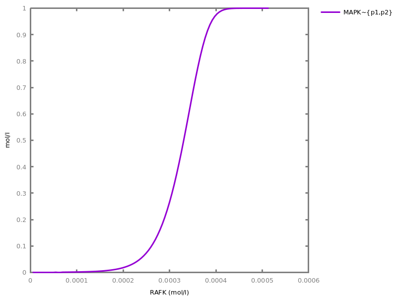
8.5. Model revision from CTL specification
This section describes commands to revise a reaction model in order to satisfy a given CTL specification of the behavior. The revision algorithm is described in [CCFS05tcsb]revise_model(Query: ctl).Use theory-revision on the current model to satisfy the query given as argument.revise_model.Use theory-revision as above, using the currently defined CTL specification.8.6. PAC Learning influence models from Boolean traces
Implementation of Leslie Valiant's PAC-Learning [doi.org/10.1215/0961754X-2872666] algoritm for k-CNF formulae [doi.org/10.1145/1968.1972], for learning influence networks from Boolean traces [CFS17cmsb].Boolean traces can be generated from Boolean simulations of a reaction or influence model, or from the stochastic simulations. Threshold values can be specified to transform a stochastic trace in a Boolean trace with the following syntax:transform ::= |nonegenerate_traces(NInitialStates: integer, timeHorizon, FilePrefix: output_file).Randomly chosesNInitialStatesinitial states and for each, runs a numerical simulation withmethod: spn,method: ssaormethod: sbnandtimeHorizonastimeoption. All results will be saved in.csvfiles with the givenFilePrefixas prefix and indexed by the run number (unless the prefix is empty).Options.
pac_learning({input_file1, ...,
        input_filen}).
Uses every time-series.csvfile in[input_file1, ..., input_filen]as source of samples to learn an influence network.Options.
- cnf_clause_size: integer
- Maximum size of CNF clauses learnt.
option(data_transform:none).option(cnf_clause_size:3).option(boolean_simulation:no).pac_learning(ModelFile: input_file, NInitialStates: integer, TimeHorizon: integer).LoadsModelFileand runsgenerate_traces/3with the provided arguments and then loads the generated files forpac_learning/1.Example. Learning Lotka-Volterra model from Boolean traces and comparison to the hidden original model.biocham:pac_learning(library:examples/lotka_volterra/LVi.bc, 200, 10, boolean_simulation: yes).% Maximum K used: 1 % minimum number of samples for h=1: 18 % 102 samples (max h ~ 5.666666666666667) P -< P % 0 samples (max h ~ 0) % _ -> P % 30 samples (max h ~ 1.6666666666666667) P,R -< R % 0 samples (max h ~ 0) % _ -> R
biocham:list_model.k1*R*P for R,P -< R. k1*R*P for R,P -> P. k2*R for R -> R. k3*P for P -< P. initial_state(R=1). initial_state(P=1). parameter( k1 = 2, k2 = 2, k3 = 1 ).
biocham:pac_learning(library:examples/circadian_cycle/bernot_comet.bc, 100, 10).% Maximum K used: 2 % minimum number of samples for h=1: 54 % 196 samples (max h ~ 3.6296296296296298) G,PC -< G % 29 samples (max h ~ 0.5370370370370371) / PC,G -> G % 456 samples (max h ~ 8.444444444444445) L -< L % 134 samples (max h ~ 2.4814814814814814) / L -> L % 176 samples (max h ~ 3.259259259259259) L,PC -< PC PC / G -< PC % 9 samples (max h ~ 0.16666666666666666) G / PC,L -> PC
biocham:list_model./ L -> L. L -< L. / G,PC -> G. G,PC -< G. G / PC,L -> PC. PC / G -< PC. PC,L -< PC.
Options.
Part III: Quantitative Analysis and Synthesis
Chapter 9
Numerical Simulations9.1. ODE and stochastic simulations
polynomial ::= monomial ::= Biocham is interfaced to the GNU Scientific Library (GSL http://www.gnu.org/software/gsl/) to perform numerical simulations. The page http://www.gnu.org/software/gsl/manual/html_node/Stepping-Functions.html#Stepping-Functions gives a detailed description of the numerical integration methods and options listed below. The implicit methodbsimpis the default one.The ODE simulation of a Biocham model proceeds by creating an ODE system if there is none, and deleting it after the simulation. It is worth noting that if there is an ODE system already present (e.g. created by import_ode), it is the current ODE system that is simulated, not the Biocham model.The stochastic simulation of a Biocham model is specific to reaction and influence models which can be interpreted by a Continuous Time Markov Chain (CTMC). The stochastic simulation algorithm cannot be directly used on an ODE system, but on an equivalent reaction system (e.g. automatically inferred with commandload_reactions_from_ode/1).method ::= |Explicit embedded Runge-Kutta (2, 3) methodrk2|Explicit 4th order (classical) Runge-Kutta. Error estimation is carried out by the step doubling method. For more efficient estimate of the error, use the embedded methods described belowrk4|Explicit embedded Runge-Kutta-Fehlberg (4, 5) method. This method is a good general-purpose integratorrkf45|Explicit embedded Runge-Kutta Cash-Karp (4, 5) method.rkck|Explicit embedded Runge-Kutta Prince-Dormand (8, 9) method.rk8pd|Implicit Gaussian first order Runge-Kutta. Also known as implicit Euler or backward Euler method. Error estimation is carried out by the step doubling method.rk1imp|Implicit Gaussian second order Runge-Kutta. Also known as implicit mid-point rule. Error estimation is carried out by the step doubling method.rk2imp|Implicit Gaussian 4th order Runge-Kutta. Error estimation is carried out by the step doubling method.rk4imp|Implicit Bulirsch-Stoer method of Bader and Deuflhard. The method is generally suitable for stiff problems.}bsimp|A variable-coefficient linear multistep Adams method in Nordsieck form. This stepper uses explicit Adams-Bashforth (predictor) and implicit Adams-Moulton (corrector) methods in P(EC)^m functional iteration mode. Method order varies dynamically between 1 and 12.msadams|Perhaps the most robust method but may be slow, a variable-coefficient linear multistep backward differentiation formula (BDF) method in Nordsieck form. This stepper uses the explicit BDF formula as predictor and implicit BDF formula as corrector. A modified Newton iteration method is used to solve the system of non-linear equations. Method order varies dynamically between 1 and 5.msbdf|Stochastic simulation of a Continuous-Time Markov Chain, defined as per Gillespie's algorithm [Gillespie76jcp]. Note that the initial concentrations are converted in molecule numbers by using thessastochastic\_conversionoption (default 100) and rounding to the nearest integer.|Stochastic Petri net simulation. Similar to the SSA algorithm above but with a discrete⁄logical time.spn|Random Petri net simulation run. All transitions are equiprobable.pn|Stochastic Boolean net simulation. Similar to the SSA algorithm above but with a discrete⁄logical time and Boolean states.sbn|Random Boolean net simulation run. All transitions are equiprobable.bn|Experimental implementation of Rosenbrock method (not compatible withrsbksearch_parametersandrobustnessandsensitivitycommands).time ::= filter ::= |Does no filtering at all.no_filter|Only keeps the points that are an extremum for some variable.only_extremaoption(method:bsimp).option(error_epsilon_absolute:1.0e-6).option(error_epsilon_relative:1.0e-6).option(initial_step_size:1.0e-6).option(maximum_step_size:0.01).option(minimum_step_size:1.0e-5).option(precision:6).option(time:20).option(steps:1).option(stochastic_conversion:100).option(stochastic_bound:1000000.0).option(stochastic_thresholding:1000).option(filter:no_filter).option(stats:no).numerical_simulation.performs a numerical simulation from time 0 up to a given time.Options.
- time: time
- time horizon of the numerical integration
- steps: integer
- number of steps at which the output is evenly sampled
- stats: yesno
- display computation time
- method: method
- method for the numerical solver
- error_epsilon_absolute: number
- absolute error for the numerical solver
- error_epsilon_relative: number
- relative error for the numerical solver
- initial_step_size: number
- initial step size for the numerical solver
- maximum_step_size: number
- maximum step size for the numerical solver, as a fraction of the total time
- minimum_step_size: number
- minimum step size, as a fraction of the total time (used to trigger events)
- precision: number
- precision for the numerical solver
- stochastic_conversion: number
- Conversion factor used to scale 1 mole to the given number of molecules (default 100).
- stochastic_bound: number
- Maximum number of molecules of one molecular species allowed in stochastic simulations (default 1e6).
- stochastic_thresholding: number
- Do not write (but still compute) stochastic steps below one fraction of the total time (default 1000)
- filter: filter
- filtering function for the trace
continue.Continues the numerical simulation by extending the time horizon by option "time" units.Options.
- time: time
- time to add to the numerical integration
9.2. Hybrid simulations
This section describes a hybrid numerical simulation method, defined either statically by distinguishing the continuous reactions from the stochastic reactions, or dynamically using a strategy based on the number of particles and velocity of the reactions. Species appearing in both continous and stochastic reactions are called hybrid species. The total particle count of one species is calculated and plotted in the simulation trace.The default simulation time is 200, and the convertion rate between particle and concentration is 1. The simulation method currently used is the Rosenbrock method.hybrid_static_simulation(ODEFilename, StochFilename).This is a hybrid simulation with a static partitioning of the reactions. The first input file contains the informations concerning the continous reactions. The second input file contains the informations concerning the stochastic reactions. Please list out all the species initial value (by initial_state(Variable = Value)) in input files.hybrid_static_simulation(ODEFilename, StochFilename, OutFilename, Volume, Time).hybrid_dynamic_simulation(InputFile, PropTresh, PartTresh).This is a hybrid simulation with a dynamic partitioning of the reactions. The input file, a normal .bc file, contains all the infomation needed. The first coefficient will be used in the propencity treshold. The second coefficient is for the particle count treshold. If a reaction meets the two conditions based on these tresholds anytime during the simulation, the reaction is seen as continuous. Otherwise, it is viewed as stochastic. Therefore, if theses numbers are high, the simulation is more precise but slower. On the contrary, the simulation is quicker but less precise if the numbers are low. Please list out all the species initial value (by initial_state(_,_)) in input files.hybrid_dynamic_simulation(InputFile, OutFilename, Volume, Time, PropTresh, PartTresh).9.3. Plotting and exporting the result of simulations
axes ::= ||x|y|xyfloatorauto ::= |autooption(plot_table:'').option(show:{}).option(logscale:'').option(against:'Time').option(xmin:auto).option(ymin:auto).option(xmax:auto).option(ymax:auto).plot.plots the current trace. After a simulation, the trace is composed of molecular concentrations and user-defined functions over time.Example.biocham:load(library:examples/mapk/mapk).biocham:numerical_simulation(method:msbdf).biocham:plot.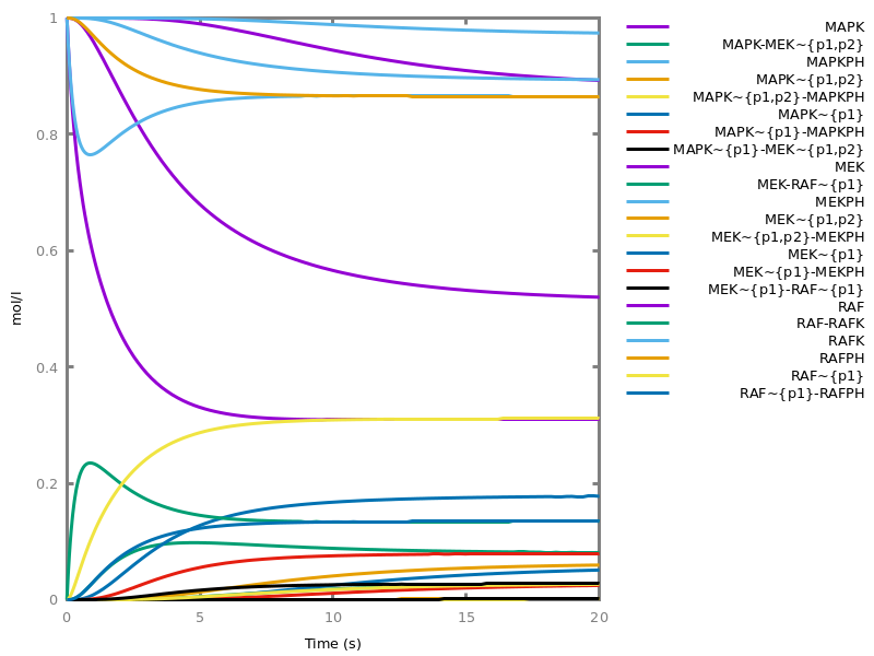
biocham:plot(show: {MAPK~{p1,p2}, MEK~{p1,p2}}).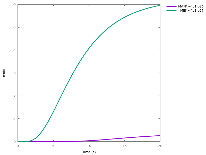
biocham:numerical_simulation(filter:only_extrema).biocham:plot.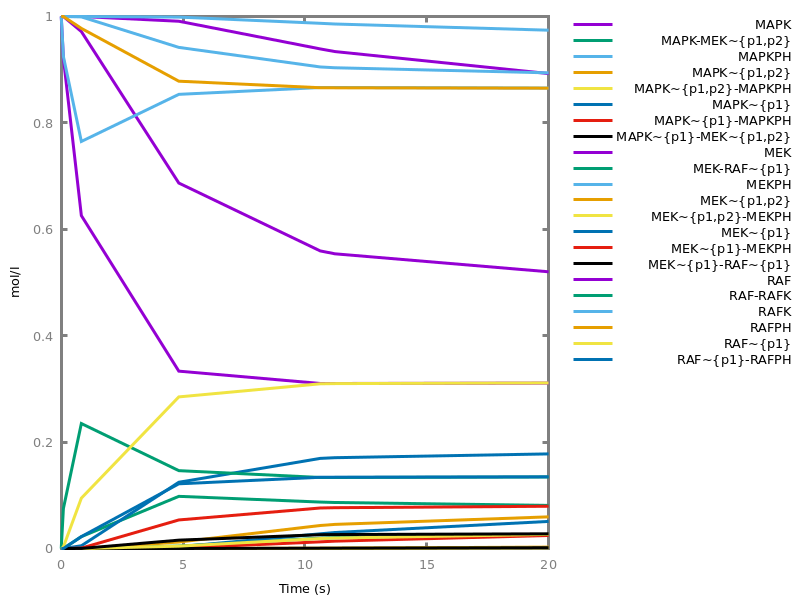
Options.
- plot_table: name
- Determined the table to be plotted
- logscale: axes
- Apply log-scaling to the specified axes.
- show: {object1, ..., objectn}
- Restricts the plot to the given set of objects and functions; everything will be plotted if the set is empty
- against: object
- Selects the X axis for the plot, defaulting to Time.
- xmin: floatorauto
- Select the axes for the current plot (auto is overwrite to *)
- ymin: floatorauto
- Select the axes for the current plot (auto is overwrite to *)
- xmax: floatorauto
- Select the axes for the current plot (auto is overwrite to *)
- ymax: floatorauto
- Select the axes for the current plot (auto is overwrite to *)
Example.biocham:a->b.biocham:a-<a.biocham:present(a,10).biocham:numerical_simulation(time:5,method:ssa).biocham:plot.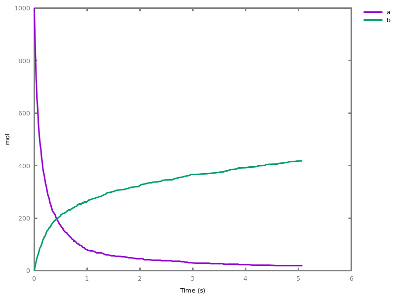
biocham:numerical_simulation(time:5,method:msbdf).biocham:plot.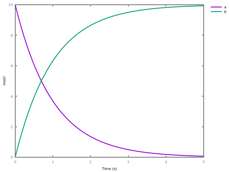
biocham:plot(logscale:y).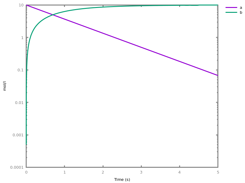
biocham:plot(show:a,against:b).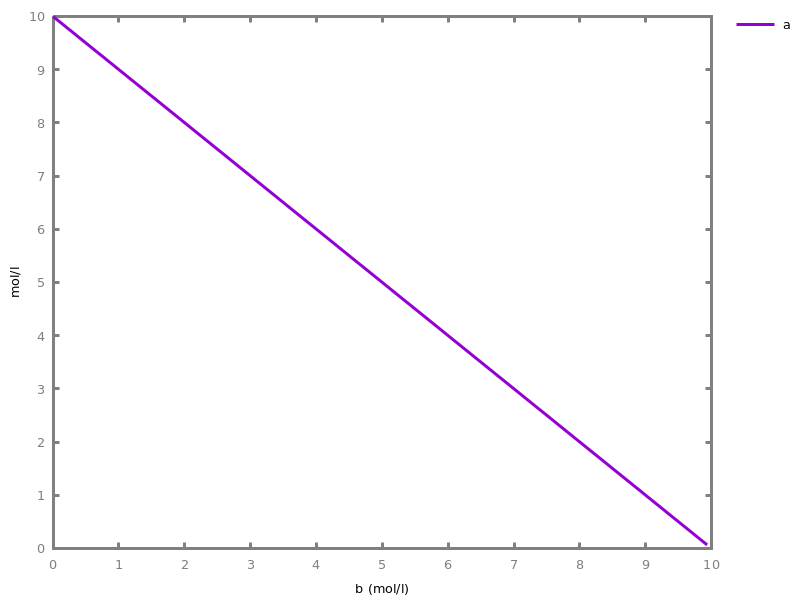
biocham:plot(show:a,against:b,logscale:xy).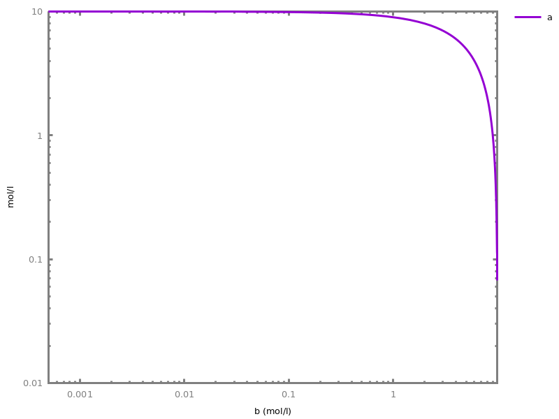
export_plot(FileTemplate: output_file).saves the current trace into two files:FileTemplate.csvand.plot.export_plot_to_png(output_file).plots the current trace in a PNG fileexport_plot_to_svg(output_file).plots the current trace in a SVG fileexport_plot_to_pdf(output_file).plots the current trace in a PDF file9.4. Variations and bifurcations
This section describes commands for continuously varying the values of molecular species or parameters.This can be used for drawing dose-response diagrams by slowly varying the dose, under the hypothesis that the input dose is a catalyst not affected itself by the system. It can also be used for drawing some simple forms of bifurcation diagrams obtained by just varying forth and back an input.variation(object, Value1: arithmetic_expression, Value2: arithmetic_expression).Makes a molecule continuously vary from Value1 to Value2 in the time option duration, under the hypothesis that the object is not affected by the other reactions on this time scale. This is achieved by adding a synthesis reaction with appropriate kinetics, removing any previous variation reaction on the object, and setting its initial concentration to Value1.Options.
- time: time
- duration of the variation.
logarithmic_variation(object, Value1: arithmetic_expression, Value2: arithmetic_expression).Makes a logarithmic variation. Value1 must be non zero.Options.
- time: time
- duration of the variation.
clear_variation(object).Deletes any variation of the object and restores its initial state.clear_variations.Deletes all variations.Example.biocham:option(time:6).biocham:variation(a,1.0e-7,0.1).biocham:logarithmic_variation(b,1.0e-7,0.1).biocham:numerical_simulation.biocham:plot.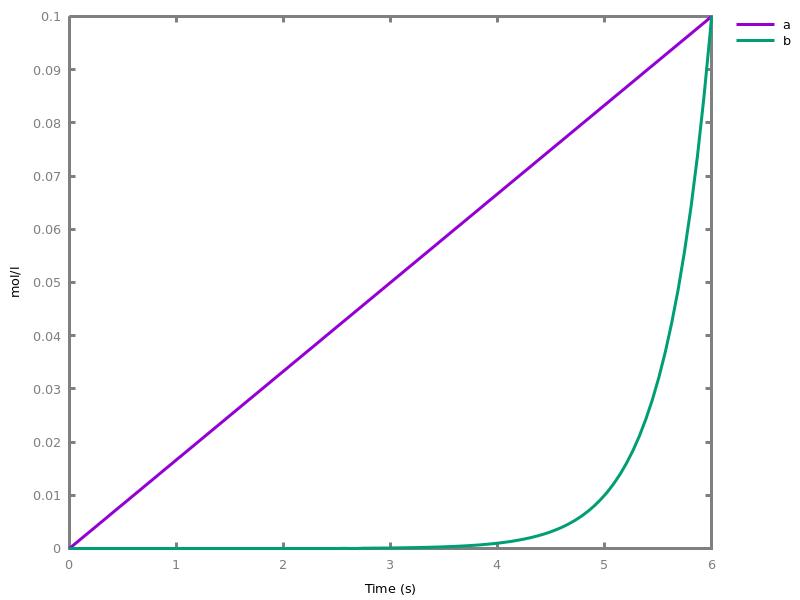
biocham:plot(logscale:y).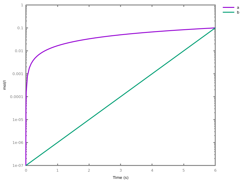
biocham:list_model.variation_a--(0.1-1.0e-7)/6 for _=>a. variation_b--b*log((1.0e-20+0.1)/(1.0e-20+1.0e-7))/6 for b=>2*b. initial_state(a=1.0e-7). initial_state(b=1.0e-7).
dose_response(Dose: object, Value1: arithmetic_expression, Value2: arithmetic_expression).Draws a dose-response diagram by linear variation of the initial concentration (the dose) of the input object which must be a catalyst not affected by the system, from Value1 to Value2, and plotting the output object (the response) in relation to the dose. A set of output objects can be given to draw their respective responses. The time option should be greater or equal to the simulation time horizon necessary to approximate the steady state response for all values of the dose. The slow variation of the dose is performed over a time horizon of 100 fold that simulation time.Options.
logarithmic_dose_response(Dose: object, Value1: arithmetic_expression, Value2: arithmetic_expression).Draws a similar dose-response diagram by logarithmic variation and plots it on a logarithmic scale for both the dose and the responses. Value1 must be non zero.Example. This example shows the dose-response diagrams of the MAPK model of Huang and Ferrell in BiomModels revealing the amplifier and analog-digital converter functions of this network at the second and third level of the cascade.biocham:load_sbml(library:biomodels/BIOMD0000000009.xml).biocham:option(time:100, show:{P_KKK,PP_KK,PP_K}).biocham:dose_response(E1,1e-6,1e-4).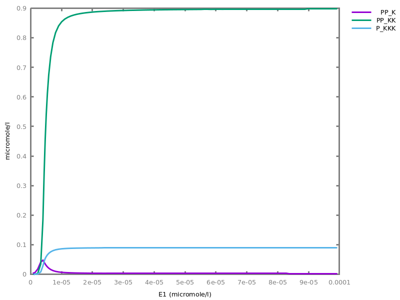
change_parameter_to_variable(Object: parameter_name).Transforms a parameter in a variable initialized to the parameter value (and creates a parameter named variation_Object). This transformation is reversible.restore_parameter(object).Restores a varying parameter to a fixed parameter.bifurcations(Dose: object, Value1: arithmetic_expression, Value2: arithmetic_expression).Draws a dose-response diagram by linear variation from Value1 to Value2 and then from Value2 to Value1 (to see memory effects) of the input object which must be a catalyst not affected by the system, and plots the output object responses. The time duration should be greater or equal to the simulation time horizon necessary to get the response at steady state (in both the increasing forward and decreasing backward variations which may be different). The slow increasing and decreasing variations of the dose are performed over a time horizon of 100 fold the simulation time. Unlike a real bifurcation diagram that draws the stable zeros of the differential function of the response, the steady states are not computed here but approximated by simulation.logarithmic_bifurcations(Dose: object, Value1: arithmetic_expression, Value2: arithmetic_expression).Draws a similar dose-response diagram by logarithmic variation using a logarithmic scale for both the dose and the response. Value1 and Value2 must be non zero.Example. This example of the MAPK network shows a memory effect in one single level of two phosphorylation cycles. The hysteresis corresponds to the existence of two stable states in the rate equation.biocham:load_sbml(library:biomodels/BIOMD0000000026.xml).biocham:dose_response(MAPKK, 0, 100, time:1e4, show:Mpp).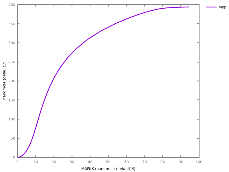
biocham:bifurcations(MAPKK, 0, 100, time:1e4, show:Mpp).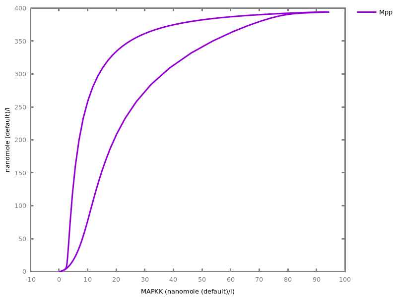
Chapter 10
Verification of Temporal Behaviors and Parameter Synthesis10.1. Numerical data time series
Numerical data time series, produced by biological experiments or by simulations, can be stored in.csvfiles, and loaded. They can also be modified by the following commands.load_table(input_file).loads the given.csvfile as a table.export_table(output_file).exports the current table into a.csvfile.list_tables.lists the current set of tables.select_table(Table: name).selectsTableto be the current table.rename_table(name).renames the current table.delete_table(name1, ..., namen).deletes some tables.list_rows.lists the rows of the current table.list_columns.lists the column names of the current table.Columns can be designated by their index or their name.delete_column(column1, ..., columnn).deletes the given columns from the current table.rename_column(column, name).renames the given column of the current table.delete_row(number1, ..., numbern).deletes the given rows from the current table.list_last_state.lists the last state of the current simulation trace.set_initial_last_state.sets the last state as new initial state.10.2. Temporal logic FO-LTL(Rlin) formulae
Firt-Order Linear Time Logic with linear constraints over the reals, FO-LTL(Rlin), can be used to specify semi-qualitative semi-quantitative properties or constraints on the dynamical behavior of the system, in a much more flexible manner than by curves to fit [RBFS11tcs]. The syntax of FO-LTL(Rlin) formulas is given below with some useful abbreviations [FT14book].FO-LTL(Rlin) formulas are evaluated on infinite traces obtained from finite traces by automatically completing them with a loop on the last state. Finite numerical data time series can be generated by simulation or loaded from biological experiment data.FO-LTL(Rlin) formulas may contain free variables, in which case they are called constraints. While a closed formula (i.e. without free variable) is either true or false on a trace, a formula with free variable is either satisfiable (i.e. true for some valuations of the variables) or unsatisfiable (i.e. false for any valuation). Verifying the satisfiability of an FO-LTL(Rlin) formula thus amounts to compute the validity domain of its variables.The symbol==tests equality of real numbers on a discrete trace by interpolation and should be prefered to exact equality=as explained and illustrated in the example below.foltl ::= |false|truefoltl_predicate ::= time_value_list ::= parameter_between_interval ::= Equality over the real numbers is the equality of floating point numbers. A predicate for equality by interpolation with next time point, notedA==B, is also defined on a discrete trace byA = B \⁄ (A > B ⁄\ X(A < B)) \⁄ (A < B ⁄\ X(A > B))i.e. the interpolation equality holds in any state satisfying just one inequality with the opposite inequality in its next state (Rolle Theorem). The interpolation equality should be used for instance when fixing theTimestate variable to a value that is not present in the trace (see example below).Thefoltl_magnitudeoption (default 5) is the multiplicative factor used for the strong comparison operators<<and>>over positive numbers,A<<Bmeans5*A<B.Thefoltl_precisionoption (default 12, i.e. $10^{-12}$) is used for converting and solving FO-LTL constraints over the integers instzead of floating point numbers.option(foltl_precision: 12).option(foltl_magnitude: 5).validity_domain(Formula: foltl).solves a FOLTL(Rlin) constraint on the current trace, i.e. computes the validity domain for the free variables that make the formula true on the numerical trace. The formula is false if the validity domain of one of its free variables is empty, and satisfiable otherwise.Example.biocham:MA(k) for A => B.biocham:present(A,a).biocham:parameter(a=1, k=1).biocham:option(time:5).biocham:numerical_simulation.biocham:plot.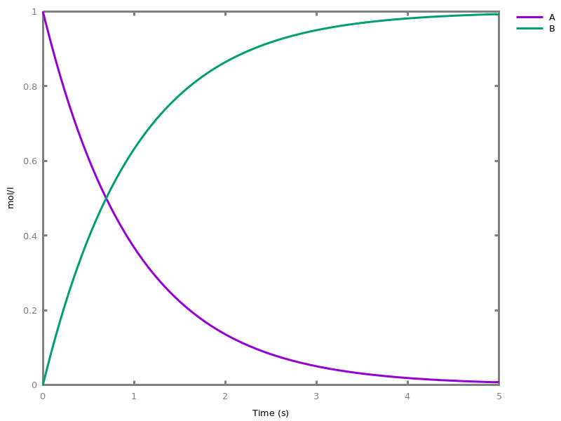
biocham:validity_domain(F(Time==1 /\ A=x /\ B=y)).x=0.371929/\y=0.628071
biocham:validity_domain(F(Time=1 /\ A=x /\ B=y)).false
biocham:validity_domain(F(Time=T /\ A==B)).T=0.689051
biocham:validity_domain(F(Time=T /\ A=B)).false
biocham:validity_domain(F(A==B /\ A=x /\ B=y)).x=0.502052/\y=0.497948
Options.
satisfaction_degree(Formula: foltl, [variable_objective1, ...,
        variable_objectiven]).
computes the continuous satisfaction degree in the interval [0,+∞) of an FOLTL(Rlin) formula on the current trace with respect to objective values given for each free variable of the formula (variables without objective should be existentially quantified in the formula). The satisfaction degree is greater or equal than 1 if the formula is satisfied. The greater the degree the greater the margin in the satisfaction of the formula (i.e. formula satisfaction robustness). This satisfaction degree is computed by (an approximation of) the distance of the objective point to the validity domain of the formula (if less than 1), or by its penetration depth (if greater than 1).Example.biocham:satisfaction_degree(F(Time==T /\ A=x /\ B=y), [T -> 0.689, x -> 0.5, y-> 0.5]).0.997106
biocham:satisfaction_degree(F(Time==T /\ A=x /\ B=y), [T -> 1, x -> 0.5, y-> 0.5]).0.877357
Options.
ltl_pattern(function_prototype1 = foltl1,
       ...,
       function_prototypen =
       foltln).
defines new F0-LTL formula patterns.list_ltl_patterns.lists all known FO-LTL formula patterns.expand_ltl(Formula: foltl).shows the expansion in FO-LTL of a formula pattern.delete_ltl_pattern(functor1, ..., functorn).deletes some LTL patterns. Either the arity is given with the pattern name⁄arity, or all LTL patterns with the given functor are deleted.Furthermore, some useful abbreviations have been predefined with the following FO-LTL(Rlin) formula patterns:ltl_pattern forall(X, Formula) = not(exists(X, not(Formula))).ltl_pattern reachable(Formula) = F(Formula).ltl_pattern steady(Formula) = G(Formula).Curves.ltl_pattern curve(Molecule, Time_Value_List) = curve(Molecule, Time_Value_list).Sequence of events [doi.org/MRMFJ08bi].ltl_pattern occurs(Formula) = F(Formula).ltl_pattern excludes(Formula) = G(not(Formula)).ltl_pattern invariates(Formula) = G(Formula).ltl_pattern weak_sequence(Formula1, Formula2) = F(Formula1 /\ F(Formula2)).ltl_pattern exact_sequence(Formula1, Formula2) = F(Formula1 /\ X(Formula2)).ltl_pattern sequence(Formula1, Formula2) = G(U(Formula1,Formula2)).ltl_pattern consequence(Formula1, Formula2) = G(Formula1 => F(Formula2)).ltl_pattern implication(Formula1, Formula2) = G(Formula1 => Formula2).Thresholds, global extrema, amplitudes [FT14book].ltl_pattern reached(Molecule, Concentration) = F(Molecule >= Concentration).ltl_pattern unreached(Molecule, Concentration) = F(Molecule <= Concentration).ltl_pattern inf_amplitude(Molecule, Amplitude) = exists(Concentration, F(Molecule <= Concentration /\ F(Molecule >= Concentration+Amplitude))).ltl_pattern sup_amplitude(Molecule, Amplitude) = exists(Concentration, G(Molecule >= Concentration /\ Molecule <= Concentration+Amplitude)).ltl_pattern first_value(Molecule, Concentration) = (Molecule=Concentration).ltl_pattern last_value(Molecule, Concentration) = F(G(Molecule=Concentration)).ltl_pattern maximum(Molecule, Concentration) = (G(Molecule <= Concentration) /\ F(Molecule>=Concentration)).ltl_pattern minimum(Molecule, Concentration) = (G(Molecule >= Concentration) /\ F(Molecule<=Concentration)).ltl_pattern maximum(Molecule, Concentration, T) = (G(Molecule <= Concentration) /\ F(Molecule>=Concentration /\ Time=T)).ltl_pattern minimum(Molecule, Concentration, T) = (G(Molecule >= Concentration) /\ F(Molecule<=Concentration /\ Time=T)).ltl_pattern amplitude(Molecule, Amplitude) = exists(Minimum, exists(Maximum, maximum(Molecule,Maximum) /\ minimum(Molecule, Minimum) /\ Amplitude=Maximum-Minimum)).Local extremaltl_pattern increase(Molecule, Concentration) = ((Molecule<=Concentration) /\ X(Molecule>=Concentration)).ltl_pattern decrease(Molecule, Concentration) = ((Molecule>=Concentration) /\ X(Molecule<=Concentration)).ltl_pattern increase(Molecule) = exists(Concentration, increase(Molecule, Concentration)).ltl_pattern decrease(Molecule) = exists(Concentration, decrease(Molecule, Concentration)).ltl_pattern local_maximum(Molecule, Concentration) = F(peak(Molecule,Concentration)).ltl_pattern local_maximum(Molecule, Concentration, T) = F(peak(Molecule,Concentration,T)).ltl_pattern peak(Molecule, Concentration) = (Molecule<Concentration /\ X(decrease(Molecule, Concentration))).ltl_pattern peak(Molecule, Concentration, T) = (Molecule<Concentration /\ X(decrease(Molecule, Concentration) /\ Time=T)).ltl_pattern first_peak(Molecule, Concentration, T) = U(decrease(Molecule), U(increase(Molecule), peak(Molecule, Concentration, T))).ltl_pattern first_peak(Molecule, Concentration) = U(decrease(Molecule), U(increase(Molecule), peak(Molecule, Concentration))).ltl_pattern last_peak(Molecule, Concentration, T) = F(peak(Molecule, Concentration, T) /\ X(U(decrease(Molecule), U(increase(Molecule), exists(c, G(Molecule=c)))))).ltl_pattern last_peak(Molecule, Concentration) = F(peak(Molecule, Concentration /\ X(U(decrease(Molecule), U(increase(Molecule), exists(c, G(Molecule=c))))))).ltl_pattern successive_peaks(Molecule, C1, T1, C2, T2) = F(U(decrease(Molecule), U(increase(Molecule), peak(Molecule,C1, T1) /\ X(first_peak(Molecule, C2, T2))))).ltl_pattern successive_peaks(Molecule, C1, C2) = F(U(decrease(Molecule), U(increase(Molecule), peak(Molecule,C1) /\ X(first_peak(Molecule, C2))))).ltl_pattern first_successive_peaks(Molecule, C1, T1, C2, T2) = U(decrease(Molecule), U(increase(Molecule), peak(Molecule,C1, T1) /\ X(first_peak(Molecule, C2, T2)))).ltl_pattern last_successive_peaks(Molecule, C1, T1, C2, T2) = F(peak(Molecule,C1, T1) /\ X(U(decrease(Molecule), U(increase(Molecule), peak(Molecule,C2, T2) /\ X(U(decrease(Molecule), U(increase(Molecule), exists(c, G(Molecule=c))))))))).ltl_pattern local_minimum(Molecule, Concentration) = F(base(Molecule,Concentration)).ltl_pattern local_minimum(Molecule, Concentration, T) = F(base(Molecule,Concentration,T)).ltl_pattern base(Molecule, Concentration) = (Molecule>Concentration /\ X(increase(Molecule, Concentration))).ltl_pattern base(Molecule, Concentration, T) = (Molecule>Concentration /\ X(increase(Molecule, Concentration) /\ Time=T)).ltl_pattern first_base(Molecule, Concentration, T) = U(increase(Molecule), U(decrease(Molecule), base(Molecule, Concentration, T))).ltl_pattern first_base(Molecule, Concentration) = U(increase(Molecule), U(decrease(Molecule), base(Molecule, Concentration))).ltl_pattern last_base(Molecule, Concentration, T) = F(base(Molecule, Concentration, T) /\ X(U(increase(Molecule), U(decrease(Molecule), exists(c, G(Molecule=c)))))).ltl_pattern last_base(Molecule, Concentration) = F(base(Molecule, Concentration /\ X(U(increase(Molecule), U(decrease(Molecule), exists(c, G(Molecule=c))))))).ltl_pattern successive_bases(Molecule, C1, T1, C2, T2) = F(U(increase(Molecule), U(decrease(Molecule), base(Molecule,C1, T1) /\ X(first_base(Molecule, C2, T2))))).ltl_pattern successive_bases(Molecule, C1, C2) = F(U(increase(Molecule), U(decrease(Molecule), base(Molecule,C1) /\ X(first_base(Molecule, C2))))).ltl_pattern first_successive_bases(Molecule, C1, T1, C2, T2) = U(increase(Molecule), U(decrease(Molecule), base(Molecule,C1, T1) /\ X(first_base(Molecule, C2, T2)))).ltl_pattern last_successive_bases(Molecule, C1, T1, C2, T2) = F(base(Molecule,C1, T1) /\ X(U(increase(Molecule), U(decrease(Molecule), base(Molecule,C2, T2) /\ X(U(increase(Molecule), U(decrease(Molecule), exists(c, G(Molecule=c))))))))).Periods and delays.ltl_pattern period(Molecule, Period) = exists(T1, exists(T2, exists(C1, exists(C2, successive_peaks(Molecule, C1, T1, C2, T2) /\ Period=T2-T1)))).ltl_pattern first_period(Molecule, Period) = exists(T1, exists(T2, exists(C1, exists(C2, first_successive_peaks(Molecule, C1, T1, C2, T2) /\ Period=T2-T1)))).ltl_pattern last_period(Molecule, Period) = exists(T1, exists(T2, exists(C1, exists(C2, last_successive_peaks(Molecule, C1, T1, C2, T2) /\ Period=T2-T1)))).ltl_pattern delay(Molecule1, Molecule2, Delay) = exists(T1, exists(T2, exists(C1, exists(C2, F(peak(Molecule1,C1,T1) /\ first_peak(Molecule2,C2,T2) /\ Delay=T2-T1))))).ltl_pattern first_delay(Molecule1, Molecule2, Delay) = exists(T1, exists(T2, exists(C1, exists(C2, U(decrease(Molecule1), U(increase(Molecule1), peak(Molecule1, C1, T1) /\ first_peak(Molecule2,C2,T2) /\ Delay=T2-T1)))))).ltl_pattern last_delay(Molecule1, Molecule2, Delay) = exists(T1, exists(T2, exists(C1, exists(C2, last_peak(Molecule1,C1,T1) /\ last_peak(Molecule2,C2,T2) /\ Delay=T2-T1)))).ltl_pattern base_period(Molecule, Period) = exists(T1, exists(T2, exists(C1, exists(C2, successive_bases(Molecule, C1, T1, C2, T2) /\ Period=T2-T1)))).ltl_pattern first_base_period(Molecule, Period) = exists(T1, exists(T2, exists(C1, exists(C2, first_successive_bases(Molecule, C1, T1, C2, T2) /\ Period=T2-T1)))).ltl_pattern last_base_period(Molecule, Period) = exists(T1, exists(T2, exists(C1, exists(C2, last_successive_bases(Molecule, C1, T1, C2, T2) /\ Period=T2-T1)))).ltl_pattern base_delay(Molecule1, Molecule2, Delay) = exists(T1, exists(T2, exists(C1, exists(C2, F(base(Molecule1,C1,T1) /\ first_base(Molecule2,C2,T2) /\ Delay=T2-T1))))).ltl_pattern first_base_delay(Molecule1, Molecule2, Delay) = exists(T1, exists(T2, exists(C1, exists(C2, U(increase(Molecule1), U(decrease(Molecule1), base(Molecule1, C1, T1) /\ first_base(Molecule2,C2,T2) /\ Delay=T2-T1)))))).ltl_pattern last_base_delay(Molecule1, Molecule2, Delay) = exists(T1, exists(T2, exists(C1, exists(C2, last_base(Molecule1,C1,T1) /\ last_base(Molecule2,C2,T2) /\ Delay=T2-T1)))).10.3. Parameter sensitivity, robustness and parameter optimization w.r.t. FO-LTL(Rlin) properties
option(robustness_coeff_var: 0.1).option(robustness_samples: 30).option(positive_sampling: yes).option(openmpi_procs: 1).The continuous satisfaction degree of an FO-LTL(Rlin) in a given trace with respect to the objective values for the free variables can be used in multiple ways: either to search parameter values in high parameter dimension to satisfy a temporal property [RBFS11tcs], or compute robustness measures and parameter sensitivity indices with respect to parameter perturbations estimated by sampling [FS18cmsb], or to visualize the landscape in two dimensions.Those commands involve numerical simulations which are executed by samplings parameter values according to a normal distribution law around their current values with a given coefficient of variation (0.1 by default), and taking absolute values (optionpositive_samplingby default). The number of parameter set samples to consider is given by the optionrobustness_samples(default 30) which will be multiplied by the number of parameters. You can use theseed/1command to try different samplings and check whether the results are similar, otherwise the number of samples should be increased.The simulations are automatically parallelized by OpenMPI. The number of processors used is given by an option (by default 0 for automatic, temporarily replaced by 1 by default because of a bug on Ubuntu)robustness(Formula: foltl, [parameter_name1, ..., parameter_namen], [variable_objective1, ..., variable_objectiven]).computes the robustness degree defined as the mean satisfaction degree (truncated to at most 1 for each parameter set sample simulation) [RBFS11tcs], of an FOLTL formulaFormula, given with a list of[variable_objective1, ..., variable_objectiven]values for the free variables of the formula (variables without any objective value should be existentially quantified) with respect to a variation of the[parameter_name1, ..., parameter_namen](i.e. extrinsic variability).The list of parameters can also be empty to measure the robustness with respect to stochastic simulations (i.e. intrinsic variability). The robustness is estimated by sampling with a normal perturbation law around the current parameter values according to the coefficient of variation option (default 0.1 i.e. 10 per cent).Example. Continuing the previous example:biocham:robustness(F(A==B /\ A=x /\ B=y), [a, k], [x -> 0.5, y-> 0.5]).On [a,k] robustness degree: 0.951512 sensitivity: 0.048488 (computation time 4.286000 s)
Options.
- time: time
- time horizon of the numerical integration
- method: method
- method for the numerical solver
- robustness_coeff_var: number
- coefficient of variation (default 0.1, i.e. 10%)
- positive_sampling: yesno
- taking the absolute values of the sampled values (default yes)
- robustness_samples: integer
- number of samples (default 30) per parameter
- openmpi_procs: integer
- Number of processors to use with OpenMPI.
- error_epsilon_absolute: number
- absolute error for the numerical solver
- error_epsilon_relative: number
- relative error for the numerical solver
- initial_step_size: number
- initial step size for the numerical solver
- maximum_step_size: number
- maximum step size for the numerical solver, as a fraction of time
- precision: number
- precision for the numerical solver
sensitivity(Formula: foltl, [parameter_name1, ...,
        parameter_namen], [variable_objective1, ...,
        variable_objectiven]).
computes sensitivity indices for each parameter in the list[parameter_name1, ..., parameter_namen], according to a normal distribution around its current value with some given coefficient of variation (default 0.1), as the mean satisfaction degree of the formulaFormulawith[variable_objective1, ..., variable_objectiven]objective values for its free variables. This command is just a shorthand for callingrobustnessrepeatedly on each single parameter in the list one at a time (i.e. OAT method based on the mean).Options.
- time: time
- time horizon of the numerical integration
- method: method
- method for the numerical solver
- robustness_coeff_var: number
- coefficient of variation of the parameters (default 0.1)
- positive_sampling: yesno
- taking the absolute values of the sampled values (default yes)
- robustness_samples: integer
- number of samples (default 30) per parameter
- openmpi_procs: integer
- Number of processors to use with OpenMPI.
- error_epsilon_absolute: number
- absolute error for the numerical solver
- error_epsilon_relative: number
- relative error for the numerical solver
- initial_step_size: number
- initial step size for the numerical solver
- maximum_step_size: number
- maximum step size for the numerical solver, as a fraction of time
- precision: number
- precision for the numerical solver
sensitivity(Formula: foltl, [variable_objective1, ...,
        variable_objectiven]).
computes the sensitivity indices of all model parameters. This command is a shorthand for calling the previous command with all parameters.Example. The command computes sensitivity indices for both parameter a and k with default coefficient of variation of 0.1:biocham:sensitivity(F(A==B /\ A=x /\ B=y), [x -> 0.5, y-> 0.5]).On [a] robustness degree: 0.953328 sensitivity: 0.046672 (computation time 3.848000 s) On [k] robustness degree: 0.985727 sensitivity: 0.014273 (computation time 3.840000 s) [a,k] by order of decreasing sensitivity.
Options.
- time: time
- time horizon of the numerical integration
- method: method
- method for the numerical solver
- robustness_coeff_var: number
- coefficient of variation of the normal law (default 0.1)
- positive_sampling: yesno
- taking the absolute values of the sampled values (default yes)
- robustness_samples: integer
- number of samples (default 30) per parameter
- openmpi_procs: integer
- Number of processors to use with OpenMPI.
- error_epsilon_absolute: number
- absolute error for the numerical solver
- error_epsilon_relative: number
- relative error for the numerical solver
- initial_step_size: number
- initial step size for the numerical solver
- maximum_step_size: number
- maximum step size for the numerical solver, as a fraction of time
- precision: number
- precision for the numerical solver
option(cmaes_init_center: no).option(cmaes_log_normal: no).option(cmaes_stop_fitness: 0.0001).search_parameters(Formula: foltl, [parameter_between_interval1, ..., parameter_between_intervaln], [variable_objective1, ..., variable_objectiven]).tries to satisfy a FO-LTL(Rlin) constraint by varying the parameters listed in[parameter_between_interval1, ..., parameter_between_intervaln]. This search command uses the stochastic optimization procedure CMA-ES (covariance matrix adaptation evolution strategy) with the continuous satisfaction degree (truncated to 1 or not according to stop option) of the given FO-LTL(Rlin) property as fitness function.Example. This command allows us to tune the kinetic parameter k to obtain a desired timing in the previous example:biocham:search_parameters(F(Time==T /\ A==B), [0 <= k <= 2], [T -> 1]).Time: 4.065 s Stopping reason: Fitness: function value -1.08e-02 <= stopFitness (1.00e-04) Best satisfaction degree: 1.010949 [0] parameter(k=0.6833050831000044)
Options.
- time: time
- time horizon of the numerical integration
- method: method
- method for the numerical solver
- error_epsilon_absolute: number
- absolute error for the numerical solver
- error_epsilon_relative: number
- relative error for the numerical solver
- initial_step_size: number
- initial step size for the numerical solver
- maximum_step_size: number
- maximum step size for the numerical solver, as a fraction of time
- precision: number
- precision for the numerical solver
- cmaes_init_center: yesno
- initialize parameter values at the center of their domain instead of their current value
- cmaes_log_normal: yesno
- search on the log of the parameters (better if very different orders of magnitude)
- cmaes_stop_fitness: number
- stop when distance to the objective is less than this value (use 0 by default and negative values in [-1,0] to maximize margins)
- openmpi_procs: integer
- Number of processors to use with OpenMPI.
search_parameters([parameter_between_interval1, ...,
        parameter_between_intervaln], [search_condition1, ...,
        search_conditionn]).
similar tosearch_parameters/3but using a list of multiple[search_condition1, ..., search_conditionn], each condition is given as a triple composed of an FOLTL formula, a list of particular parameters instantiations (e.g. describing a mutant), and objective values for the variables of the FOLTL formula.Example.biocham:ka for _ => a.biocham:kb for _ => b.biocham:parameter(ka=1, kb=1).biocham:search_parameters([0 <= ka <= 3], [(G(a-b<x/\b-a<x), [], [x -> 10]), (G(a-b<y/\b-a<y), [kb=2], [y -> 10])]).Time: 5.058 s Stopping reason: Fitness: function value 4.68e-06 <= stopFitness (1.00e-04) Best satisfaction degree: 0.999995 [0] parameter(ka=1.5000002341053575)
Options.
- time: time
- time horizon of the numerical integration
- method: method
- method for the numerical solver
- error_epsilon_absolute: number
- absolute error for the numerical solver
- error_epsilon_relative: number
- relative error for the numerical solver
- initial_step_size: number
- initial step size for the numerical solver
- maximum_step_size: number
- maximum step size for the numerical solver, as a fraction of time
- precision: number
- precision for the numerical solver
- cmaes_init_center: yesno
- initialize parameter values at the center of their domain instead of their current value
- cmaes_log_normal: yesno
- search on the log of the parameters (better if very different orders of magnitude)
- cmaes_stop_fitness: number
- stop when distance to the objective is less than this value (use negative to enforce robustness)
- openmpi_procs: integer
- Number of processors to use with OpenMPI.
option(resolution: 10).scan_parameters(Formula: foltl, Parameter1: parameter_between_interval, Parameter2: parameter_between_interval, [variable_objective1, ..., variable_objectiven]).returns some statistics and draws the landscape of the satisfaction degrees (truncated to 1) of a FO-LTL(Rlin) formula obtained by varying two parameters in intervals given, possibly on loagarithmic scale. Note that the number of calls to numerical integration is the square of the resolution option valueN. By default the image and the data are saved in fileslandscape_Parameter1_Parameter2_N.pngand.txtrespectively. Note that the drawing shows an overapproximation of the best values found for the parameters. The precise values are available in filelandscape_Parameter1_Parameter2_N.txt.Example.biocham:MA(k)for a => b. present(a,10).biocham:MA(l) for b => a.biocham:scan_parameters(F(Time > T /\ a > b), (0 <= k <= 2), (0 <= l <= 2), [T -> 5], resolution:3).Time: 28.999 s Mean satisfaction (robustness): 0.380110, standard deviation: 0.584952 Maximum satisfaction: 1.000000 Best solutions found with 0.000000<=k<=1.000000, 0.000000<=l<=2.000000
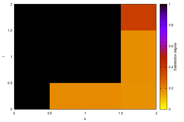
Options.
- logscale: axes
- parameter sampling and axes on a logarithmic scale
- resolution: number
- number of values tried for each parameter (default is 10)
- time: time
- time horizon of the numerical integration
- method: method
- method for the numerical solver
- error_epsilon_absolute: number
- absolute error for the numerical solver and minimum value on logarithmic scale
- error_epsilon_relative: number
- relative error for the numerical solver
- initial_step_size: number
- initial step size for the numerical solver
- maximum_step_size: number
- maximum step size for the numerical solver, as a fraction of time
- precision: number
- precision for the numerical solver
- openmpi_procs: integer
- Number of processors to use with OpenMPI.
scan_parameters(Formula: foltl, Parameter1: parameter_between_interval, Parameter2: parameter_between_interval, [variable_objective1, ...,
        variable_objectiven], Filename: output_file).
specifies in addition to save the image in filefilename.pngand the data in filefilename.txt.Options.
- logscale: axes
- sampling and axes on a logarithmic scale
- resolution: number
- number of values tried for each parameter (default is 10)
- time: time
- time horizon of the numerical integration
- method: method
- method for the numerical solver
- error_epsilon_absolute: number
- absolute error for the numerical solver
- error_epsilon_relative: number
- relative error for the numerical solver
- initial_step_size: number
- initial step size for the numerical solver
- maximum_step_size: number
- maximum step size for the numerical solver, as a fraction of time
- precision: number
- precision for the numerical solver
- openmpi_procs: integer
- Number of processors to use with OpenMPI.
Chapter 11
Synthesis of Reaction Networks11.1. Synthesis from mathematical expressions and simple programs
In this simple program syntax each statement must be terminated by ',' or '.'.statement ::= assignment ::= variable ::= expression ::= The support of arithmetic_expression is not complete, but most of them are supported. Statements terminated by ',' will execute parallelly with next statement.lhs ::= rhs ::= control_flow_keyword ::= |if_tag|When using these two keywords, the rhs serves as the condition.while|else_tag|endif|When using these three keywords, the rhs does not matter.endwhileThe operators 'pre' and 'post' are used to describe the procedural structure of a program, so if not specified, the list element will execute parallelly, which makes it possible to describe sequential and parallel part of a program.To mix the sequential and parallel computation, statements which executed parallelly need to add 'para' before the expression, except the last statement.Currently it is user's responsibility to ensure the execution of last statement finishs after other parallelly executed statements.add_function(term1 = term1, ..., termn = termn).adds reactions to compute the result of a function of the current variables in the concentration of a new variable, at steady state. This command only accepts input list with each element of this form: <lhs> = <rhs>.Example.biocham:present(x,1).biocham:present(y,3).biocham:add_function(z=x+y).biocham:list_ode.[0] d(z_p)/dt=x_p+y_p-z_p-fast*z_n*z_p [1] d(z_n)/dt=x_n+y_n-z_n-fast*z_n*z_p [2] d(x_p)/dt=0 [3] d(y_p)/dt=0 [4] d(x_n)/dt=0 [5] d(y_n)/dt=0 [6] d(x)/dt=0 [7] d(y)/dt=0 [8] d(temp0_p)/dt=0 [9] d(temp0_n)/dt=0 [10] d(temp1_p)/dt=0 [11] d(temp1_n)/dt=0 [12] init(z_p=0) [13] init(z_n=0) [14] init(x_p=1) [15] init(y_p=3) [16] init(x_n=0) [17] init(y_n=0) [18] init(x=1) [19] init(y=3) [20] init(temp0_p=0) [21] init(temp0_n=0) [22] init(temp1_p=0) [23] init(temp1_n=0) [24] par(fast=1000)
biocham:list_model.MA(1) for x_p=>x_p+z_p. MA(1) for y_p=>y_p+z_p. MA(1) for z_p=>_. MA(1) for x_n=>x_n+z_n. MA(1) for y_n=>y_n+z_n. MA(1) for z_n=>_. MA(fast) for z_n+z_p=>_. initial_state(x=1). initial_state(y=3). initial_state(temp0_p=0). initial_state(temp0_n=0). initial_state(temp1_p=0). initial_state(temp1_n=0). initial_state(x_p=1). initial_state(x_n=0). initial_state(y_p=3). initial_state(y_n=0). initial_state(z_p=0). initial_state(z_n=0). parameter( fast = 1000 ).
biocham:numerical_simulation(time:10).biocham:plot.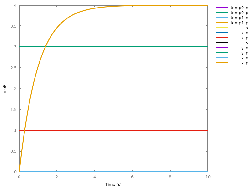
Options.
- zero_ultra_mm: yesno
- set the kinetics of zero-order ultrasensitivity to Michaelis-Menten kinetics
option(simplify_variable_init:no).option(zero_ultra_mm:no).compile_program(Program: atom).Using atom Program as the program code.We can write the follwing program and compile it in reactions.biocham:compile_program('z := 2. x := z + 1. y := x - z.',zero_ultra_mm:yes).biocham:numerical_simulation(time:60).biocham:plot(show:{x_p,x_n,y_p,y_n,z_p,z_n}).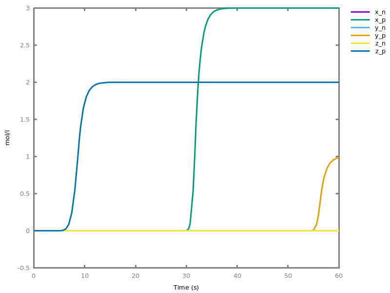 This is equivalent to '
add_function( z = ( 2 post ), x = ( pre z + 1 post ), y = ( pre x - z )).' and can be compared with the parallel version of the program, without pre and post conditions.biocham:clear_model.biocham:compile_program('z := 2, x := z + 1, y := x - z.',zero_ultra_mm:yes).biocham:numerical_simulation(time:20).biocham:plot(show:{x_p,x_n,y_p,y_n,z_p,z_n}).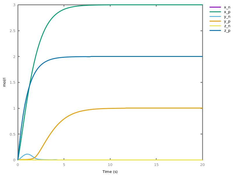
Options.
compile_program_file(input_file).Compile the high-level language program from file.Options.
11.2. Synthesis from polynomial differential equations
The Turing completeness of continuous CRNs [FLBP17cmsb] states that any computable function over the reals can be computed by a CRN over a finite set of molecular species. Biocham uses the proof of that result to compile any computable real function presented as the solution of a polynomial differential equation system with polynomial initial values (PIVP) into a finite CRN.The compilation from mathematical expression is restricted to some standard functions and simple operations using a functional notation whereidrepresents the operand.The compilation from PIVPs is implemented with full generality.The option for quadratic reduction restricts the synthesis to reactions with at most two reactants (the default is not, since this process may be costly). Two methods are available to perform this a posteriori reduction: natively or using an external SAT solver.option(quadratic_reduction:fastnSAT).option(quadratic_bound:carothers).Another option is the lazy introduction of molecular species for negative real values (the default is yes).option(lazy_negatives:yes).option(negation_first:yes).compile_from_expression(Expr: arithmetic_expression, Output: name).creates a biochemical reaction network such that Output = Expr(time). The expression is restricted to standard functions and simple operations using a functional notation whereidrepresents the time operand.Options.
- quadratic_reduction: reduction_methods
- Determine if the quadratic reduction for synthesizing reactions with at most two reactants has to be performed
- quadratic_bound: reduction_bounds
- Use the bound from Carother's article or that from Bychkov and Pogudin
- lazy_negatives: yesno
- Switch between systematic and lazy introduction of molecular species for negative values
- negation_first: yesno
- Determine if the negation of variables is perform before or after the quadratization
compile_from_expression(Expr: arithmetic_expression, Input: name, Output: name).creates a biochemical reaction network to compute the function Output = Expr(Input). The expression is restricted to standard functions and simple operations using a functional notation whereidrepresents the operand. The Input species is initialized with the value of a special parameter named input. This species may be degraded by the computation.Options.
- quadratic_reduction: reduction_methods
- Determine if the quadratic reduction for synthesizing reactions with at most two reactants has to be performed
- quadratic_bound: reduction_bounds
- Use the bound from Carother's article or that from Bychkov and Pogudin
- lazy_negatives: yesno
- Switch between systematic and lazy introduction of molecular species for negative values
Example. Compilation of the expression 4+time^2:biocham:compile_from_expression(4+id*id,output).biocham:list_model.MA(1.0) for D=>D+H+output. MA(1.0) for F=>F+H+output. MA(1.0) for _=>D+F. initial_state(output=4). initial_state(I=4). parameter( fast = 1000 ).
biocham:numerical_simulation(time:4).biocham:plot.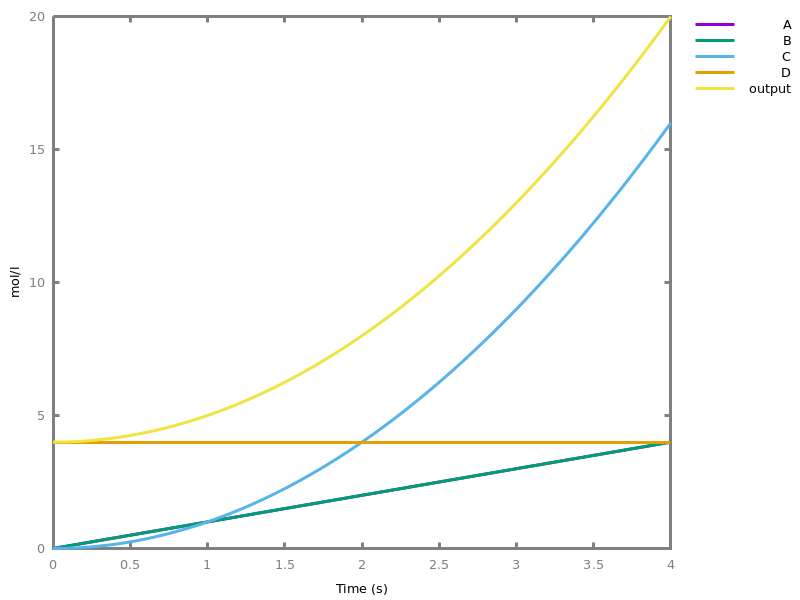 Example. Compilation of the expression cos(time):
biocham:compile_from_expression(cos,costime).biocham:list_model.MA(fast) for costime_m+costime_p=>_. MA(fast) for J_m+J_p=>_. MA(1.0) for J_p=>J_p+costime_p. MA(1.0) for J_m=>J_m+costime_m. MA(1.0) for costime_m=>J_p+costime_m. MA(1.0) for costime_p=>J_m+costime_p. initial_state(costime_p=1). parameter( fast = 1000 ).
biocham:numerical_simulation(time:10).biocham:plot.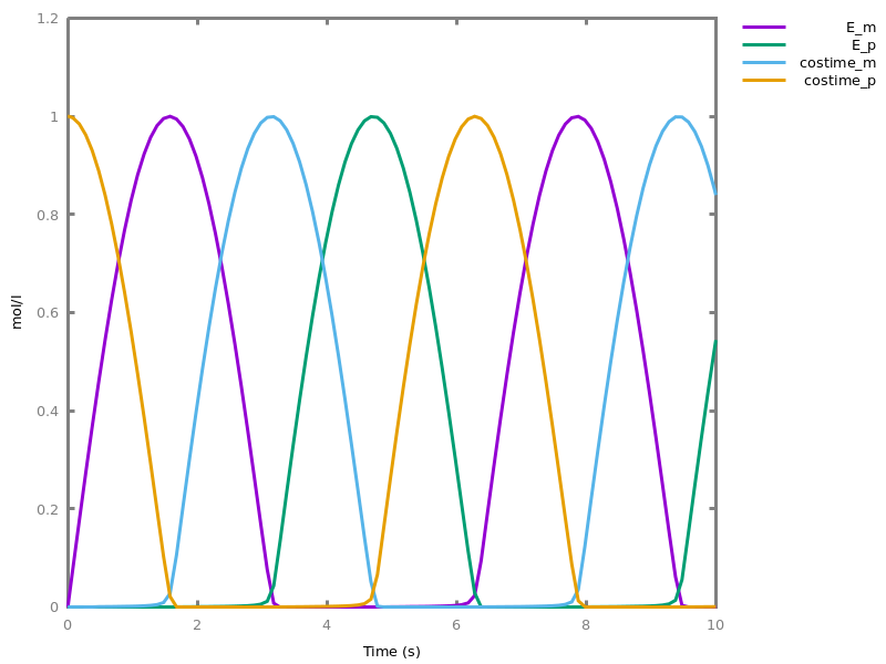 Example. Compilation of the expression cos(time):
biocham:compile_from_expression(cos+1,costime1).biocham:list_model.MA(fast) for costime1_m+costime1_p=>_. MA(fast) for N_m+N_p=>_. MA(fast) for K_m+K_p=>_. MA(1.0) for K_p=>K_p+N_p+costime1_p. MA(1.0) for K_m=>K_m+N_m+costime1_m. MA(1.0) for N_m=>K_p+N_m. MA(1.0) for N_p=>K_m+N_p. initial_state(costime1_p=2). initial_state(N_p=1). initial_state(J=1). parameter( fast = 1000 ).
biocham:numerical_simulation(time:10).biocham:plot.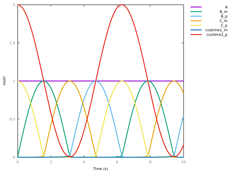 Example. Compilation of the expression cos(x) and computation of cos(4):
biocham:compile_from_expression(cos,x,cosx).biocham:list_model.MA(fast) for cosx_m+cosx_p=>_. MA(fast) for K_m+K_p=>_. MA(1.0) for K_p+x=>K_p+cosx_p+x. MA(1.0) for K_m+x=>K_m+cosx_m+x. MA(1.0) for cosx_m+x=>K_p+cosx_m+x. MA(1.0) for cosx_p+x=>K_m+cosx_p+x. MA(1.0) for x=>_. initial_state(cosx_p=1). initial_state(x=input). parameter( input = 1.0, fast = 1000 ).
biocham:parameter(input=4).biocham:numerical_simulation(time:10).biocham:plot.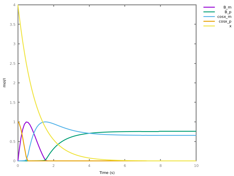 One can also compile real valued functions defined as solutions of Polynomial Initial Value Problems (PIVP), i.e. solutions of polynomial differential equations with initial values defined by polynomials of the input. PIVPs are written with the following grammar:
pode ::= compile_from_pivp(PIVP: pivp, name1, ..., namen).creates a CRN that immplements a function of time, specified by the variable "Output" of the solution of the PIVP.Options.
- quadratic_reduction: reduction_methods
- Determines if the quadratic reduction has to be performed
- quadratic_bound: reduction_bounds
- Use the bound from Carother's article or that from Bychkov and Pogudin
Example. Compilation of the Hill function of order 2 as a function of time, $h(t)=t^2⁄(1+t^2)$biocham:option(quadratic_reduction:native).biocham:compile_from_pivp((0.0,d(h)/dt=2*n^2*t;1.0,d(n)/dt= -2*n^2*t;0.0,d(t)/dt=1),[h]).biocham:list_model.MA(2.0) for n+nt=>h+nt. MA(1.0) for n=>n+nt. MA(2.0) for 2*nt=>nt. initial_state(n=1.0). parameter( fast = 1000, input = 4 ).
biocham:numerical_simulation(time:10).biocham:plot(show:{h}).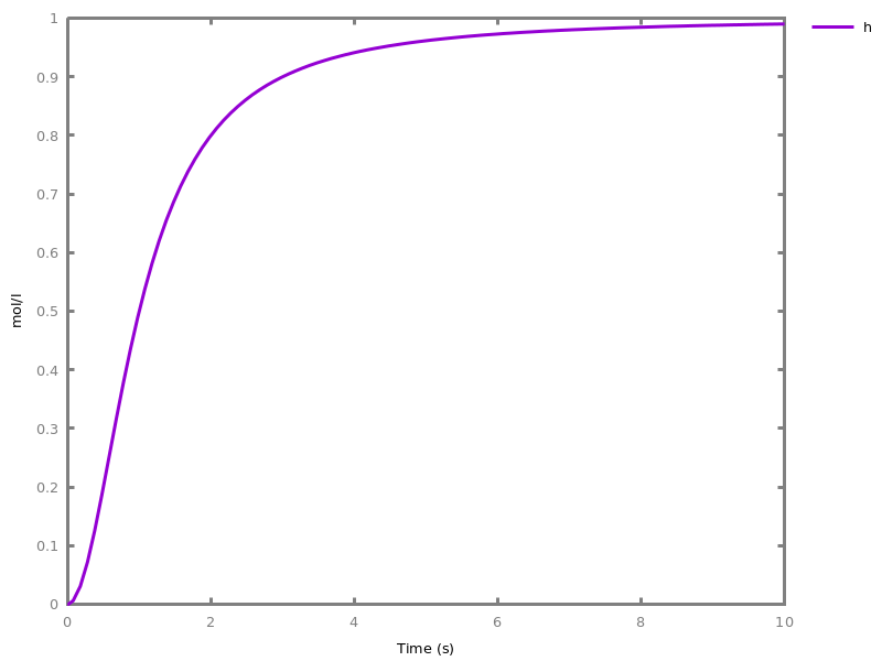
biocham:plot(show:{h},logscale:x).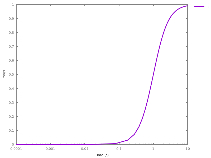
compile_from_pivp(PIVP: pivp, Input: name, name1,
       ...,
       namen).
creates a CRN that implements a function of the variable "Input". The function is specified by the value of the variable "Output" of the solution of a PIVP at time "Input". The "Input" variable must not appear in the PIVP. It is created and initialized with a parameter named "input".Options.
- quadratic_reduction: reduction_methods
- Determines if the quadratic reduction has to be performed
- quadratic_bound: reduction_bounds
- Use the bound from Carother's article or that from Bychkov and Pogudin
compile_from_ode(Input: name, name1,
       ...,
       namen).
Compile the current ODE system in a CRN, Input is usually "time" but could be the name of a new species, Output have to be the name of an existing variable.Options.
- quadratic_reduction: reduction_methods
- Determines if the quadratic reduction has to be performed
- quadratic_bound: reduction_bounds
- Use the bound from Carother's article or that from Bychkov and Pogudin
- lazy_negatives: yesno
- Switch between systematic and lazy introduction of molecular species for negative values
Example. Compilation of the Hill function of order 2 as a function of an input $h(x)=x^2⁄(1+x^2)$. This timesat_speciesis used (minimizing the number of variables as is the case fornative) and thensat_reactionsthat minimizes the number of monomes.biocham:option(quadratic_reduction:sat_species).biocham:compile_from_pivp((0.0,d(h)/dt=2*n^2*t;1.0,d(n)/dt= -2*n^2*t;0.0,d(t)/dt=1),x,[h]).biocham:parameter(input=2).biocham:list_model.MA(1.0) for x=>_. MA(2.0) for n+ntx=>h+ntx. MA(1.0) for nx=>_. MA(2.0) for ntx+nx=>ntx. MA(1.0) for nx+x=>ntx+nx+x. MA(1.0) for ntx=>_. MA(2.0) for 2*ntx=>ntx. initial_state(x=input). initial_state(n=1.0). initial_state(nx=input). parameter( fast = 1000, input = 2 ).
biocham:numerical_simulation(time:10).biocham:plot(show:{h}).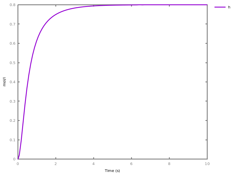
biocham:plot(show:{h},logscale:x).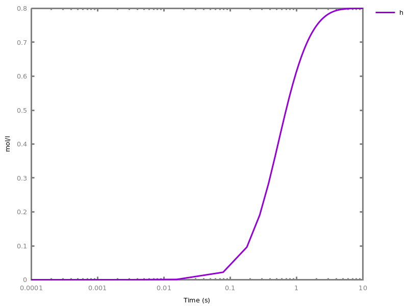
biocham:compile_from_pivp((0.0,d(h)/dt=2*n^2*t;1.0,d(n)/dt= -2*n^2*t;0.0,d(t)/dt=1),x,[h],quadratic_reduction:sat_reactions).biocham:list_model.MA(1.0) for x=>_. MA(2.0) for n+ntx=>h+ntx. MA(1.0) for nx=>_. MA(2.0) for ntx+nx=>ntx. MA(1.0) for nx+x=>ntx+nx+x. MA(1.0) for ntx=>_. MA(2.0) for 2*ntx=>ntx. initial_state(x=input). initial_state(n=1.0). initial_state(nx=input). parameter( fast = 1000, input = 1.0 ).
reduction_methods ::= |no|native|fast|fastnSAT|sat_species|sat_reactionsreduction_bounds ::= |carothers|bychkovquadratize_ode(object1, ..., objectn).Modify the ODE system in order to make it quadratic while keeping the prescribed variablespolynomial_ODE.Check if the current ODE system is polynomialcompile_function(Formula, Input: object).Compile the desired formula into a CRN by determining a corrsponding IVP, then PIVP and finally a CRN. Typical usage looks like: - compile_function(Y=f(X), X). Which set up a CRN such that when parameter(input=X), the final value of Y is f(X). and - compile_function(Y=f(Time), Time). Which set up a function of time.Options.
- quadratic_reduction: reduction_methods
- Determine if the quadratic reduction for synthesizing reactions with at most two reactants has to be performed
polynomialize_ode.Starting from the current ODE system, builds an equivalent polynomial ODE system by introducing more variables that compute the non-polynomial terms.Example. Polynomialization of an ODE system:biocham:d('A')/dt=exp('A').biocham:polynomialize_ode.B = exp(A)
biocham:list_ode.[0] d(B)/dt=B^2 [1] d(A)/dt=B [2] init(B=1.0) [3] init(A=0)
stabilize_expression(Expression: arithmetic_expression, Output: name, Point).Construct a CRN such that the Output species will adjust its concentration to satisfy the algebraic Expression in the vicinity of Point.Example. Compilation of a CRN to stabilize the Bring radical:biocham:stabilize_expression(y^5+y-x,y,[x=2,y=1]).biocham:list_model.MA(1.0) for x=>x+y. MA(1.0) for y=>_. MA(1.0) for y+y4=>y4. MA(1.0) for 2*y=>y2+2*y. MA(1.0) for y2=>_. MA(1.0) for 2*y2=>y4+2*y2. MA(1.0) for y4=>_. initial_state(x=2). initial_state(y=1). initial_state(y2=1). initial_state(y4=1). parameter( fast = 1000, input = 1.0 ).
biocham:option(time:100,show:{y}).biocham:dose_response(x,0,4).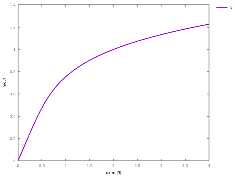
11.3. Synthesis from GPAC circuits
Biocham can compile a GPAC circuit (Shannon's General Purpose Analog Computer) into an abstract CRN using positive as well as negative concentration values. Only weak GPACs, in which the integration gate is with respect to time and not a variable, are considered. The variables associated to the different points of the circuits can be named with the "::" operator. Dy default they are named x0, x1,... The syntax of weak GPAC circuits is as follows:The option fast rate (defaulting to 1000) is intended to define a high rate constant for reactions faster than the other reactions. It is used- in the reactions for computing the results of the sum and product GPAC blocks,
- and in the annihilation reactions between the molecular species for the positive and negative values of a real valued variable.
option(fast_rate:1000).compile_wgpac({wgpac1, ..., wgpacn}).compiles a set of weak GPAC circuits into a reaction network.Options.
- fast_rate: arithmetic_expression
Example. Compilation of a GPAC circuit generating cosine as a function of time (using positive and negative concentrations) :biocham:compile_wgpac(f::integral integral-1*f).biocham:present(f,1).biocham:list_model.fast*[x2]*[f] for f+x2=>f+x1+x2. fast*[x1] for x1=>_. MA(1) for x1=>x0+x1. MA(1) for x0=>f+x0. initial_state(x2= -1). initial_state(f=1). parameter( fast = 1000 ).
biocham:numerical_simulation(time:10).biocham:plot.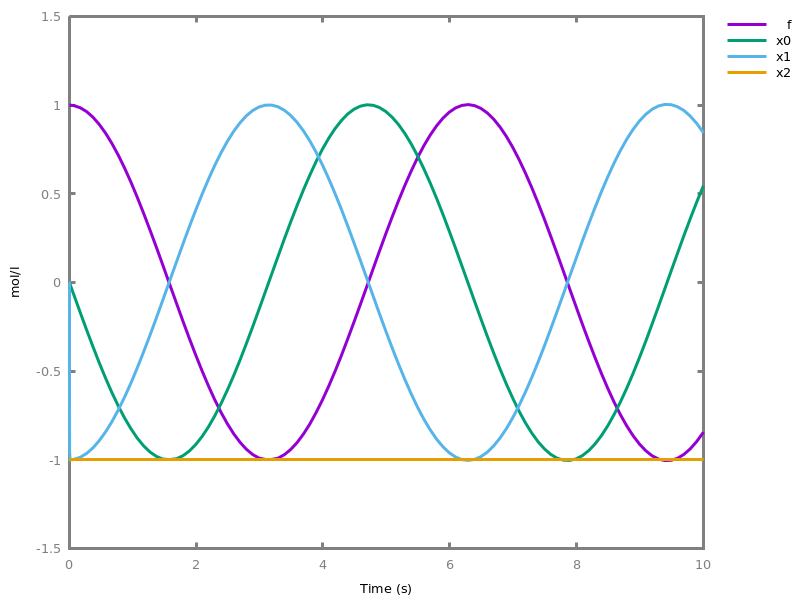
11.4. Synthesis from transfer functions
transfer_polynomial ::= |stransfer_function ::= enable_p_m_mode.Each variable corresponds to two species: one for the negative part and one for the positive part.disable_p_m_mode.Each variable corresponds to one species.which_p_m_mode.Displays which mode is being used.set_p_m_rate(Rate: number).Set the annihilation rate between two complementary species.set_kinetics_rate(Rate: number).Set the final summator ratecompile_transfer_function(F: transfer_function, U: object, Y: object).compile a transfer function in variable s into a chemical filter.compile_transfer_function([number1, ..., numbern], [number1, ..., numbern], U: object, Y: object).compile a transfer function into a chemical filter.Example.biocham:set_kinetics_rate(1000).biocham:compile_transfer_function([22,51,47,19,3],[30,66,67,36,10,1],a,b).biocham:present(a).biocham:numerical_simulation(method:msbdf).biocham:plot.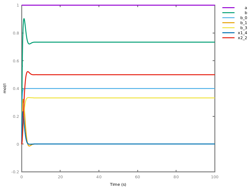
Part IV: Index of Commands
A
- about/0 1.3.
- absent/1 2.2.
- add/1 6.1.
- add_biocham/1 6.1.
- add_conservation/1 7.3.
- add_ctl/1 8.2.
- add_edge/* 3.5.
- add_event/* 5.
- add_function/* 11.1.
- add_ginml/1 6.2.
- add_influence/1 4.1.
- add_influences_from_ode/1 6.3.
- add_influences_from_ode_system/0 6.3.
- add_model_from_ode/1 6.3.
- add_ode/* 6.3.
- add_qual/1 6.2.
- add_reaction/1 3.3.
- add_reactions_from_ode/1 6.3.
- add_reactions_from_ode_system/0 6.3.
- add_sbml/1 6.2.
- add_time_event/* 5.
- add_vertex/* 3.5.
- against (option) 9.3.
- alias/1 3.2.
- all_reductions (option) 7.4.
B
- bifurcations/3 9.4.
- boolean_initial_states (option) 8.2.8.3.8.3.
- boolean_semantics (option) 8.1.8.3.8.3.8.3.
- boolean_simulation (option) 8.6.8.6.
- boolean_state_display (option) 8.1.8.1.8.3.8.3.
- boolean_trace (option) 8.3.8.3.
C
- canonical/1 3.2.
- change_parameter_to_variable/1 9.4.
- check_conservations/0 7.3.
- check_ctl/0 8.3.
- check_ltl/1 8.3.
- check_model/0 6.1.
- check_multistability/0 7.7.
- check_oscillations/0 7.7.
- check_polynomiality/0 6.1.
- cleanup_ctl/0 8.2.
- clear_ctl/0 8.2.
- clear_dimension/1 7.2.
- clear_dimensions/0 7.2.
- clear_initial_state/0 2.2.
- clear_model/0 6.1.
- clear_ode_systems/0 6.3.
- clear_variation/1 9.4.
- clear_variations/0 9.4.
- cmaes_init_center (option) 10.3.10.3.
- cmaes_log_normal (option) 10.3.10.3.
- cmaes_stop_fitness (option) 10.3.10.3.
- cnf_clause_size (option) 8.6.8.6.
- compile_from_expression/2 11.2.
- compile_from_expression/3 11.2.
- compile_from_ode/2 11.2.
- compile_from_pivp/2 11.2.
- compile_from_pivp/3 11.2.
- compile_function/2 11.2.
- compile_program/1 11.1.
- compile_program_file/1 11.1.
- compile_transfer_function/3 11.4.
- compile_transfer_function/4 11.4.
- compile_wgpac/1 11.3.
- conservation_size (option) 7.3.7.3.
- continue/0 9.1.
- correct_model/0 6.1.
D
- data_transform (option) 8.6.8.6.
- delete_alias/1 3.2.
- delete_attribute/2 3.5.
- delete_column/* 10.1.
- delete_conservation/1 7.3.
- delete_conservations/0 7.3.
- delete_ctl/1 8.2.
- delete_edge/* 3.5.
- delete_events/0 5.
- delete_function/* 2.4.
- delete_graph/1 3.5.
- delete_ltl_pattern/* 10.2.
- delete_ode/* 6.3.
- delete_ode_system/1 6.3.
- delete_parameter/* 2.3.
- delete_reaction/1 3.3.
- delete_reaction_named/1 3.3.
- delete_reaction_prefixed/1 3.3.
- delete_reactions/0 3.3.
- delete_row/* 10.1.
- delete_table/* 10.1.
- delete_temporary_files/0 1.3.
- delete_vertex/* 3.5.
- disable_p_m_mode/0 11.4.
- distinct_species (option) 7.4.
- dose_response/3 9.4.
- double_michaelis_menten (option) 7.5.
- download_curated_biomodel/1 6.2.
- draw_first (option) 3.4.
- draw_graph/0 3.4.
- draw_influence_hypergraph/0 4.2.
- draw_influences/0 4.2.
- draw_neighborhood/0 2.1.
- draw_reactions/0 3.4.
- draw_rules/0 3.4.
E
- enable_p_m_mode/0 11.4.
- enzyme (option) 7.5.
- ep (option) 7.5.
- error_epsilon_absolute (option) 9.1.10.3.10.3.10.3.10.3.10.3.10.3.10.3.
- error_epsilon_relative (option) 9.1.10.3.10.3.10.3.10.3.10.3.10.3.10.3.
- evaluate/1 2.4.
- expand_ctl/1 8.2.
- expand_ltl/1 10.2.
- export_biocham/1 6.1.
- export_graph/1 3.4.
- export_lemon_graph/1 4.2.
- export_nusmv/1 8.3.
- export_ode/1 6.3.
- export_ode_as_latex/1 6.3.
- export_plot/1 9.3.
- export_plot_to_pdf/1 9.3.
- export_plot_to_png/1 9.3.
- export_plot_to_svg/1 9.3.
- export_sbml/1 6.2.
- export_table/1 10.1.
- export_xpp/1 6.3.
- extremal_sepi (option) 7.4.
F
- fast_rate (option) 11.3.
- filter (option) 9.1.
- foltl_magnitude (option) 10.2.10.2.
- foltl_precision (option) 10.2.10.2.
- force_graph (option) 4.2.
- function/* 2.4.
G
H
- help/1 1.1.
- hill_reaction (option) 7.5.
- hybrid_dynamic_simulation/3 9.2.
- hybrid_dynamic_simulation/6 9.2.
- hybrid_static_simulation/2 9.2.
- hybrid_static_simulation/5 9.2.
I
- import_ode/1 6.3.
- import_reactions_from_graph/0 3.4.
- import_reactions_with_inhibitors (option) 6.3.6.3.6.3.6.3.
- infer_hidden_molecules (option) 6.3.6.3.
- infer_hidden_molecules/0 6.3.
- influence_graph/0 4.2.
- influence_hypergraph/0 4.2.
- influence_model/0 4.1.
- inherits/* 6.1.
- init/* 6.3.
- initial_state/* 2.2.
- initial_step_size (option) 9.1.10.3.10.3.10.3.10.3.10.3.10.3.10.3.
K
- keep_temporary_files/0 1.3.
L
- lazy_negatives (option) 11.2.11.2.11.2.
- left_to_right (option) 3.4.
- list_aliases/0 3.2.
- list_attributes/1 3.5.
- list_columns/0 10.1.
- list_conservations/0 7.3.
- list_ctl/0 8.2.
- list_current_models/0 6.1.
- list_dimensions/0 7.2.
- list_edges/0 3.5.
- list_events/0 5.
- list_functions/0 2.4.
- list_graph_objects/0 3.5.
- list_graphs/0 3.5.
- list_influences/0 4.1.
- list_initial_state/0 2.2.
- list_input_species/0 7.1.
- list_isolated_vertices/0 3.5.
- list_last_state/0 10.1.
- list_locations/0 2.1.
- list_ltl_patterns/0 10.2.
- list_model/0 6.1.
- list_models/0 6.1.
- list_molecules/0 2.1.
- list_neighborhood/0 2.1.
- list_ode/0 6.3.
- list_ode_systems/0 6.3.
- list_options/0 1.3.
- list_parameters/0 2.3.
- list_reactions/0 3.3.
- list_reactions_with_autocatalyst/1 3.3.
- list_reactions_with_catalyst/1 3.3.
- list_reactions_with_inhibitor/1 3.3.
- list_reactions_with_product/1 3.3.
- list_reactions_with_reactant/1 3.3.
- list_reactions_with_species/1 3.3.
- list_reactions_with_strict_catalyst/1 3.3.
- list_rows/0 10.1.
- list_rules/0 3.3.
- list_sink_species/0 7.1.
- list_source_species/0 7.1.
- list_stable_states/0 8.1.
- list_strict_input_species/0 7.1.
- list_tables/0 10.1.
- list_tscc_candidates/0 8.1.
- list_units/0 7.2.
- load/1 6.1.
- load_biocham/1 6.1.
- load_ginml/1 6.2.
- load_influences_from_ode/1 6.3.
- load_influences_from_ode_system/0 6.3.
- load_model_from_ode/1 6.3.
- load_qual/1 6.2.
- load_reactions_from_ode/1 6.3.
- load_reactions_from_ode_system/0 6.3.
- load_sbml/1 6.2.
- load_table/1 10.1.
- logarithmic_bifurcations/3 9.4.
- logarithmic_dose_response/3 9.4.
- logarithmic_variation/3 9.4.
- logscale (option) 9.3.10.3.10.3.
- ltl_pattern/* 10.2.
M
- make_absent_not_present/0 2.2.
- make_present_not_absent/0 2.2.
- mapping_restriction (option) 7.4.
- max_nb_reductions (option) 7.4.
- maximum_step_size (option) 9.1.10.3.10.3.10.3.10.3.10.3.10.3.10.3.
- merge_reactions/2 3.3.
- merge_restriction (option) 7.4.
- method (option) 9.1.10.3.10.3.10.3.10.3.10.3.10.3.10.3.
- michaelis_menten (option) 7.5.
- michaelis_menten_expansion (option) 7.5.
- minimum_step_size (option) 9.1.
- multistability_graph/0 4.2.
N
- negation_first (option) 11.2.
- new_graph/0 3.5.
- new_model/0 6.1.
- new_model/1 6.1.
- new_ode_system/0 6.3.
- numerical_simulation/0 9.1.
- nusmv_topological_order (option) 8.3.
O
- ode_function/* 6.3.
- ode_parameter/* 6.3.
- ode_system/0 6.3.
- openmpi_procs (option) 10.3.10.3.10.3.10.3.10.3.10.3.10.3.
- option/0 1.3.
- output_to_library (option) 6.2.
P
- pac_learning/1 8.6.
- pac_learning/3 8.6.
- parameter/* 2.3.
- parametrize/0 6.1.
- partial_hill_reaction (option) 7.5.
- pathway/2 7.1.
- pattern_reduction/2 7.5.
- place/* 3.5.
- plot/0 9.3.
- plot_table (option) 9.3.
- polynomial_ODE/0 11.2.
- polynomialize_ode/0 11.2.
- positive_sampling (option) 10.3.10.3.10.3.
- precision (option) 9.1.10.3.10.3.10.3.10.3.10.3.10.3.10.3.
- present/1 2.2.
- present/2 2.2.
- prolog/1 1.3.
Q
- quadratic_bound (option) 11.2.11.2.11.2.11.2.11.2.
- quadratic_reduction (option) 11.2.11.2.11.2.11.2.11.2.11.2.
- quadratize_ode/* 11.2.
- query (option) 8.3.
- quit/0 1.3.
R
- r_1 (option) 7.5.
- r_2 (option) 7.5.
- reaction_graph/0 3.4.
- reaction_model/0 4.1.
- read_xpp/1 6.3.
- reduce_model/0 8.4.
- reduce_model/1 8.4.
- remove_fraction/0 6.3.
- rename_column/2 10.1.
- rename_table/1 10.1.
- reset_options/0 1.3.
- resolution (option) 10.3.10.3.
- restore_parameter/1 9.4.
- revise_model/0 8.5.
- revise_model/1 8.5.
- robustness/3 10.3.
- robustness_coeff_var (option) 10.3.10.3.10.3.
- robustness_samples (option) 10.3.10.3.10.3.
- rule_graph/0 3.4.
S
- satisfaction_degree/2 10.2.
- scan_parameters/4 10.3.
- scan_parameters/5 10.3.
- search_conservations/0 7.3.
- search_efms/0 7.3.
- search_parameters/2 10.3.
- search_parameters/3 10.3.
- search_reduction/2 7.4.
- second_order_closure (option) 6.3.
- seed/1 1.3.
- select_graph/1 3.5.
- select_model/1 6.1.
- select_ode_system/1 6.3.
- select_table/1 10.1.
- sensitivity/2 10.3.
- sensitivity/3 10.3.
- set_attribute/2 3.5.
- set_dimension/3 7.2.
- set_graph_name/1 3.5.
- set_initial_last_state/0 10.1.
- set_kinetics_rate/1 11.4.
- set_model_name/1 6.1.
- set_ode_system_name/1 6.3.
- set_p_m_rate/1 11.4.
- set_units/2 7.2.
- show (option) 9.3.9.4.9.4.9.4.9.4.
- show_support (option) 7.4.
- simplify_variable_init (option) 11.1.11.1.
- stabilize_expression/3 11.2.
- stats (option) 7.4.7.6.9.1.
- steps (option) 9.1.
- stochastic_bound (option) 9.1.
- stochastic_conversion (option) 9.1.
- stochastic_thresholding (option) 9.1.
T
- test_permutations (option) 7.7.
- test_rate_independence/0 7.8.
- test_rate_independence_invariants/0 7.8.
- test_stochastic_mean_ode/0 7.9.
- test_transpositions (option) 7.7.
- time (option) 9.1.9.1.9.4.9.4.9.4.9.4.9.4.9.4.10.3.10.3.10.3.10.3.10.3.10.3.10.3.
- timeout (option) 7.4.
- transition/* 3.5.
- tropical_denominator (option) 7.6.
- tropical_epsilon (option) 7.6.
- tropical_ignore (option) 7.6.
- tropical_max_degree (option) 7.6.
- tropical_single_solution (option) 7.6.
- tropicalize/0 7.6.
U
V
W
X
Y
Z